Branching circuits experiment

My good friend and motion graphics bromance, Eli Guerron, asked me to help him create a procedural system of branching circuits that would look something like a schematic drawing. I stupidly thought this would be an easy trick with particles, but to get the right look it actually took quite a lot of experimenting.

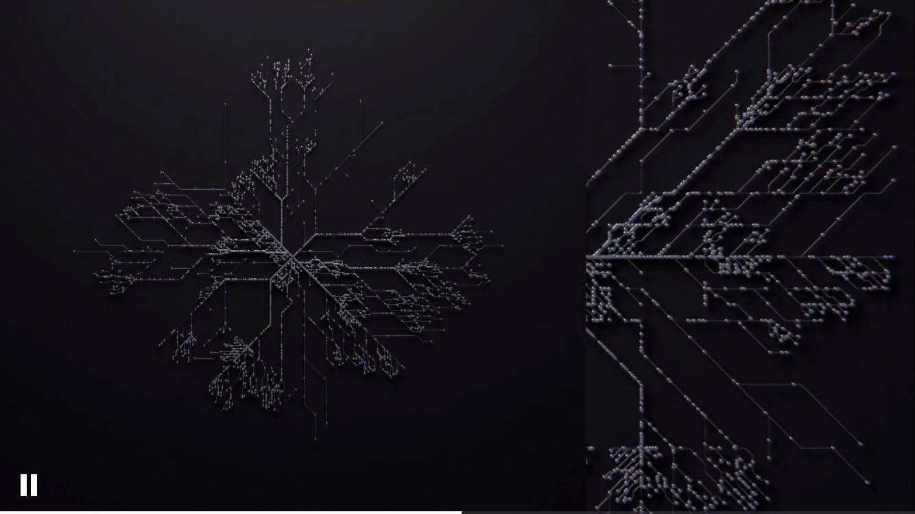
The reference video he showed me showed branching structures that would occasionally turn or split apart at precise angles. This part was easy enough to figure out, but the real trick was preventing collisions between branches. I first thought that I could use a modified version of the space colonization algorithm to create the non-intersecting patterns, but even after writing a function to restrict the growth directions to increments of 45 degrees (explained below), I couldn’t get the patterns to look right. Part of the reason the reference image looks “schematic-y” is because the traces will run alongside each other in parallel, sometimes splitting apart but generally running in groups. Space colonization just doesn’t grow that way, so I had to throw that method out.

The method that worked the best (it’s still not perfect) is just growing polylines in a SOP Solver, completely manually in VEX snippets. Each point has a starting velocity vector (this is left over from when I originally tried to solve this with particles), and on each timestep the endpoints will duplicate themselves, then add their velocity to their point position, and draw a polyline between the original and the duplicate. This forms the basis of the traces. The code for this is pretty straightforward:

// create new point, inheriting attrs from this point
int newpt = addpoint(0,@ptnum);
// assign new position to new point
vector newv = normalize(v@v) * speed;
vector newpos = @P + (newv);
setpointattrib(0,"P",newpt,newpos,"set");
setpointattrib(0,"v",newpt,newv,"set");
// add primitive to connect new point to current point
int newprim = addprim(0,"polyline");
addvertex(0,newprim,@ptnum);
addvertex(0,newprim,newpt);
// remove old point from "growth" group...
// this can be done by just setting a point attribute

The next step is to get the traces to randomly zigzag at 45 degree angles. Since I’m dealing with vectors here, rotating vectors is most easily done (IMO) via a matrix. The math really isn’t too bad, but there’s a few steps that need to happen to make this work.

First, I need to create a generic identity matrix. This is just a matrix for the point that, when multiplied against the point position (or any other vector attribute, such as velocity), returns the same vector right back. Creating an identity matrix is easy:

matrix3 m = ident();

Next, I want to generate an angle of 45 degrees. When dealing with vector math in general, you typically want radians, not degrees. 45 degrees is equivalent to π/4 radians, which I can then randomly negate to create either a positive or negative angle.

matrix3 m = ident();
float PI = 3.14159;
float angle = (PI * 0.25);
if(rand(@ptnum*@Time+seed) < 0.5) {
    angle *= -1;
}

Now I need to define an axis to rotate my angle around. Since my schematic is growing on the XZ plane, the axis to bend around would be the Y axis, or the vector {0,1,0}. Once I have the axis, the angle, and a matrix, I can use VEX’s rotate() function to rotate my identity matrix. All you have to do at that point is multiply any vector by that matrix, and it will rotate to the specified angle. Keep in mind that for predictable results, your vector should be normalized before multiplying it against a rotation (3×3) matrix. You can always multiply the resulting vector against the length of the original vector, once you’re done.

matrix3 m = ident();
float PI = 3.14159;
float angle = (PI * 0.25);
if(rand(@ptnum*@Time+seed) < 0.5) {
    angle *= -1;
}
vector up = {0,1,0};
rotate(m,angle,up);
newv = (normalize(newv) * m) * speed;
setpointattrib(0,"v",newpt,newv,"set");

The branching step is almost exactly the same. I just randomly generate a new point and rotate its velocity by +/- 45 degrees, but don’t remove the original point from the growth group. (In my example HIP, the “tips” growth group is defined by being red, while the static group is green. The “tips” group is redefined at the beginning of each step based on color.)

This setup alone gets some pretty cool patterns, but it’s messy without collision detection:

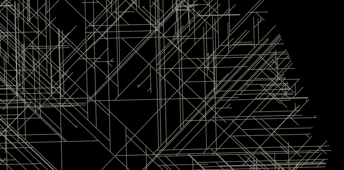
The collision detection is where things get tricky. I wanted growth points to look ahead of themselves along their velocity vector, and if they detected a collision, to try to match the collision surface’s velocity. This process repeats in a loop until the point can verify that nothing is blocking future growth. If the loop exceeds a maximum number of tries, it kills the branch by removing the point from the growth group.

The easiest way to “look ahead” and grab the velocity from collided polylines was to use the intersect() function. This returns a primitive number (or -1 if there was no collision), and parametric UV coordinates at the collision site. The primitive number and UV coordinates can then be fed into the primuv() function, which can be used to grab any attribute value at those exact coordinates. The velocity value at the collision point can then be assigned to the growth point so it moves in the same direction.

// find intersection along velocity vector.
// if an intersection is found, inherit that point's
// velocity attribute.
// repeat this up to "maxtries" to resolve collisions.
// if there is still a collision when maxtries is reached,
// remove this particle from the tips group (turn green).

vector interP;
vector forward = {1,0,0};
vector up = {0,1,0};
float PI = 3.14159;
float interU;
float interV;
int maxtries = chi("max_tries");
int try = 0;

while(try <= maxtries) {
    int primnum = intersect(1,@P,v@v*4,interP,interU,interV);
    if(primnum != -1) {
        // we collided
        // get velocity of collision point
        vector uv = set(interU,interV,0);
        vector collideV = primuv(1,"v",primnum,uv);
        v@v = collideV;
        // if this was the last try, this line has to stop
        if(try==maxtries) {
            // turn green to remove from tips on next step
            @Cd = {0,1,0};
        }
    }
    try+=1;
}

This works… okay, but because the points sometimes collide in between points that are at angles to each other, every once in a while the primuv() function will return angles that are a little “fuzzy,” meaning not at 45-degree angles. It doesn’t happen often, but when it does happen, you start seeing some weird curvy lines. So as a last step, the velocity vectors need to be locked to 45-degree angles, just in case.

First, I define a forward and up vector. Forward is +X (1,0,0), up is +Y (0,1,0). The forward vector is to have an axis to compare the velocity against… since this schematic is being drawn on the XZ plane, the +X axis is just a convenient starting point for figuring out rotations. To rotate angles on this XZ plane, I use the Y axis (up).

Figuring out the angle between two vectors is straightforward. The formula is this:

float theta = acos( dot(V1,V2) );

This returns the angle (typically called theta) between vectors V1 and V2, in radians. Because of the way this calculation works, it’s only going to properly return angles for vectors pointing towards +Z, so if the velocity has a negative Z component, we just multiply the angle by -1.

float angle = acos( dot( normalize(v@v),forward) );
if(v@v.z < 0) {
    angle *= -1;
}

Next, we need to figure out how far away our angle is from a 45-degree angle. We can do this by using the modulo operator to figure out the remainder when we divide our angle by (π/4).

float angle = acos( dot( normalize(v@v),forward) );
float rem = angle % (PI * 0.25);
angle -= rem;
if(v@v.z < 0) {
    angle *= -1;
}

Now we have a nice 45-degree-divisible angle relative to +X (or 0 radians). We need to turn this into a unit vector, which we can then multiply against our original velocity vector’s length to get the final velocity.

Check out this circle diagram to see what we’re doing here:

Substitute Y with Z and you can already see the exact formula we’re going to use. Thanks to the unit circle, we can easily plot out where on the circle we’ll be with a little more trig. Then we just have to multiply that against the original velocity’s magnitude (length).

float angle = acos( dot( normalize(v@v),forward) );
float rem = angle % (PI * 0.25);
angle -= rem;
if(v@v.z < 0) {
    angle *= -1;
}
vector newV = set(cos(angle),0,sin(angle)) * length(v@v);
v@v = newV;

The final result is pretty cool! I still don’t like how some of the branches get too close to each other, and points can still intersect each other when two tips collide with each other on the same point, but it’s pretty close to the original setup. I’d like to eventually figure out a better way to keep the spacing between traces a little more consistent (right now they tend to sometimes bunch up tighter than I’d like), but that will have to happen later on.

Here’s the HIP file, if you want to play with it!