Texturing flowing liquids

One of the bigger challenges with rendering liquids is that it can be difficult to get good UVs on them for texturing. Getting a displacement map on a liquid sim can make all the difference when you need some added detail without grinding out a multimillion-particle simulation. Unfortunately, liquid simulations have the annoying habit of stretching your projected UVs out after just a few seconds of movement, especially in more turbulent flows.

In Houdini smoke and pyro simulations, there’s an option to create a “dual rest field” that acts as an anchor point for texturing so that textures can be somewhat accurately applied to the fluid and they will advect through the velocity field. The trick with dual rest fields is that they will regenerate every N seconds, offset from each other by N/2 seconds. A couple of detail parameters called “rest_ratio” and “rest2_ratio” are created, which are basically just sine waves at opposite phases to each other, used as blending weights between each rest field. When it’s time for the first rest field to regenerate, its blend weight is at zero while the rest2 field is at full strength, and vice versa.

It’s great that these are built into the smoke and pyro solvers, but of course nothing in Houdini can be that easy, so for FLIP simulations we’ll have to do this manually. Rather than dig into the FLIP solver and deal with microsolvers and fields, I’ll do this using SOPs and SOP Solvers in order to simplify things and avoid as many DOPs nightmares as possible.

Here’s the basic approach: Create two point-based UV projections from the most convenient angle (XZ-axis in my case) and call them uv1 and uv2. As point attributes, they’ll automatically be advected through the FLIP solver. Then reproject each UV map at staggered intervals, so that uv2 always reprojects halfway between uv1 reprojections. We’ll also create a detail attribute to act as the rest_ratio which will always be 0 when uv1 is reprojecting, and 1 when uv2 is reprojecting. It all sounds more complicated than it really is. Here goes…

Let’s assume you already have a FLIP simulation that moves more or less the way you want it. Inside the DOP network, connect the output of the FLIP solver to the green input of a MultiSolver, then rewire the FLIP Object to the gray input of the MultiSolver. We’re going to create a SOP Solver and connect it to the green input of the MultiSolver and arrange it so that it happens after the FLIP solve. (See Fig. 1.)

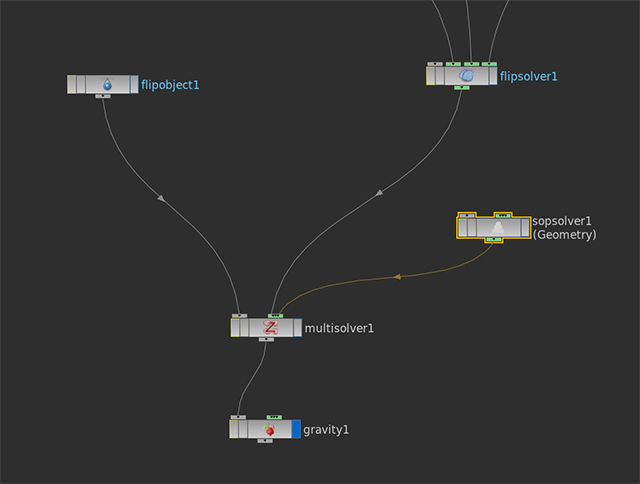
Fig. 1. The DOP network connections. Note that the FLIP Object is connected to the Multi Solver, not the FLIP Solver.

Next, dive into the SOP Solver. The first purple node should be called “dop_geometry,” and this will output the state of the DOP simulation at the current frame. What we want to do is reproject UVs, but ONLY if we’re at the right frame. In order to make this easier to control later on, I like to create a parameter that’s very visible and easy to remember for later. Create a null and put a channel on it called “rate” or “rest_time” or really whatever you want. Mine’s called “rate.” Make it an integer and set it to 2. This means that each UV set will reproject every 2 seconds.

We’re going to use an Attribute Wrangle SOP to actually do all the logic work. Connect the “dop_geometry” to the first input of an Attribute Wrangle. Next, create a UVTexture SOP and connect it to the output of the “dop_geometry” as well. The exact projection type and axis depends on your individual simulation; I’m using Y-axis. This node gets connected to the second input of the Attribute Wrangle.

Our logic is this: if we’re at a time (in seconds) divisible by our “rate” parameter, reproject uv1. If we’re at a time where time + (rate*0.5) is divisible by “rate,” reproject uv2. This means both sets regenerate at the same rate, but halfway between each other. Now we just have to translate this to CVEX. The code looks like this:


float rate = ch("../CONTROL/rate");
if( (@Time % rate) == 0) {
v@uv1 = point(1,"uv",@ptnum);
}
if( ((@Time + (rate * 0.5)) % rate) == 0) {
v@uv2 = point(1,"uv",@ptnum);
}


The first line there defines the variable “rate” as being equal to the parameter created on the null. This could point anywhere, depending on what your channel is named, or you could define it explicitly here (although this will make other parts of this setup more difficult later). Next, if time modulo the rate is 0 (meaning it’s cleanly divisible), set uv1 to be equal to the “uv” attribute of the second input (which is input index 1 in the point expression). The last condition does the same thing for uv2, but with a time offset equal to half the rate in order to stagger the projections.

Next up, we have to generate the “rest_ratio” detail parameter. I’m creating this as a detail parameter in this case because that’s what the Pyro solver does, even though later on we’ll be converting it to a point attribute in order to make it accessible in a VOP SOP. Create a new detail float attribute and call it “rest_ratio,” but don’t set it to anything yet. We’ll use a CHOPnet to generate the wave. We could do this with an expression, but I like doing things visually and seeing the CHOP works better for me. Make a CHOPnet and dive inside. Lay down a Wave CHOP and set its period parameter to be equal to your “rate” attribute… use a relative reference for this, so ch("../../CONTROL/rate"). Set the phase to 0.25, so the curve starts at 0, and set the offset to 1 and the amplitude to 0.5 so that the curve goes from 0 to 1 instead of -1 to 1. Connect this channel to a Null CHOP named “OUT” and then jump back out. Set the value of rest_ratio to this expression: chop("../chopnet1/OUT/chan1") (your channel or CHOPnet names might be different, substitute those in). Your final SOP Solver network should look something like Figure 2.

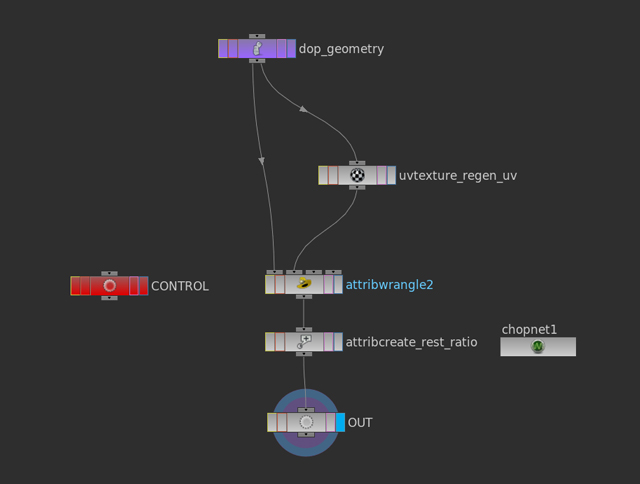
Fig. 2. The SOP Solver network. The “CONTROL” is just a Null with a parameter on it that we can reference for both the Attribute Wrangle and the CHOPNet.

Almost there. Now we have to use these parameters in shading. For a faster preview, though, we can apply textures to point colors in SOPs. The process for setting up the material in SHOPs and assigning point colors are about the same, so it should be trivial to translate this to shading.

Go back to the SOPs context, to whatever point in your scene you are importing the DOP geometry. This is probably after an auto-generated DOP Import SOP somewhere. The first thing we’ll do is promote rest_ratio to a point attribute so we can access it quickly in a VOP SOP. Next, create a VOP SOP and dive inside. The logic here is simple: import both uv1 and uv2 attributes, lookup the value of a color map at the given UV coordinates for each set, and then blend them together using the rest_ratio as the bias for the color mix.

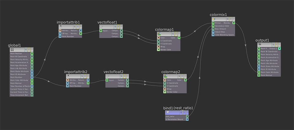
Fig. 3. The VOP SOP network for blending colors from two UV sets, biased by the rest_ratio parameter.

Dive inside the VOP SOP. Create two Import Attribute VOPs, and set the Attribute to uv1 and uv2, respectively. Connect each of them to a Vector to Float VOP. Create a pair of Color Map VOPs, and set the Color Map parameter for each to “$HH/pic/UVcolor.rat,” or any other color map you feel like using. For each Color Map VOP, connect the first and second outputs of the Vector to Float VOPs to the U and V coordinate inputs. Create a Color Mix VOP and connect the first Color Map VOP to Primary Color, and the second to Secondary. Import the “rest_ratio” attribute, and then connect it to the “Bias” attribute of the Color Mix VOP. Then just output the Color Mix to Point Color (Cd).

If your connections are right, you should see the two color maps blending together so that the texture never “snaps” as it is reprojected. Here’s an example:

You can see that 2 seconds between reprojections is probably a bit fast, but thankfully that number is easily adjusted. You could even to a second set of projections (uv3 and uv4) at a faster or slower rate, and use the relative velocity of the particles to blend between fast reprojections and slow reprojections.