Another year, another very very short side project. This was meant to be both an exploration of Vellum (and an attempt to see if I could force Vellum to work in 2D), and a neat little intro video for a new demo reel. This project is considerably less complicated than the rainy forest cinemagraph project I documented last year, but I hope reading the breakdown here is still informative.
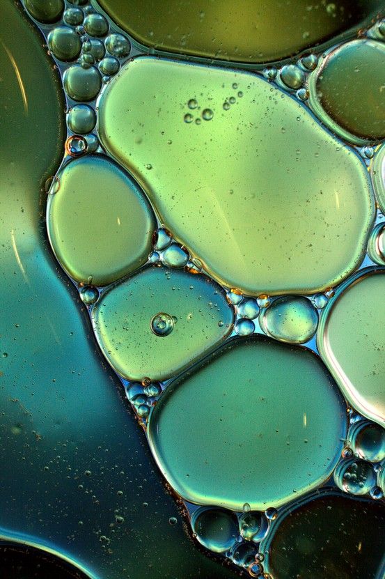
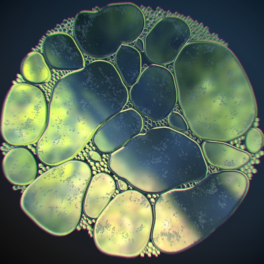
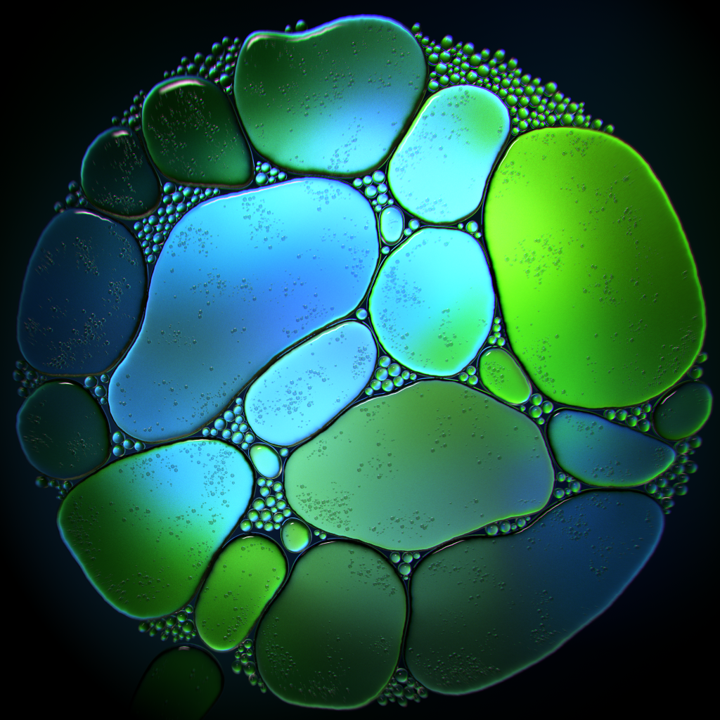
The goal of this project was to somehow recreate this photo, but in motion:
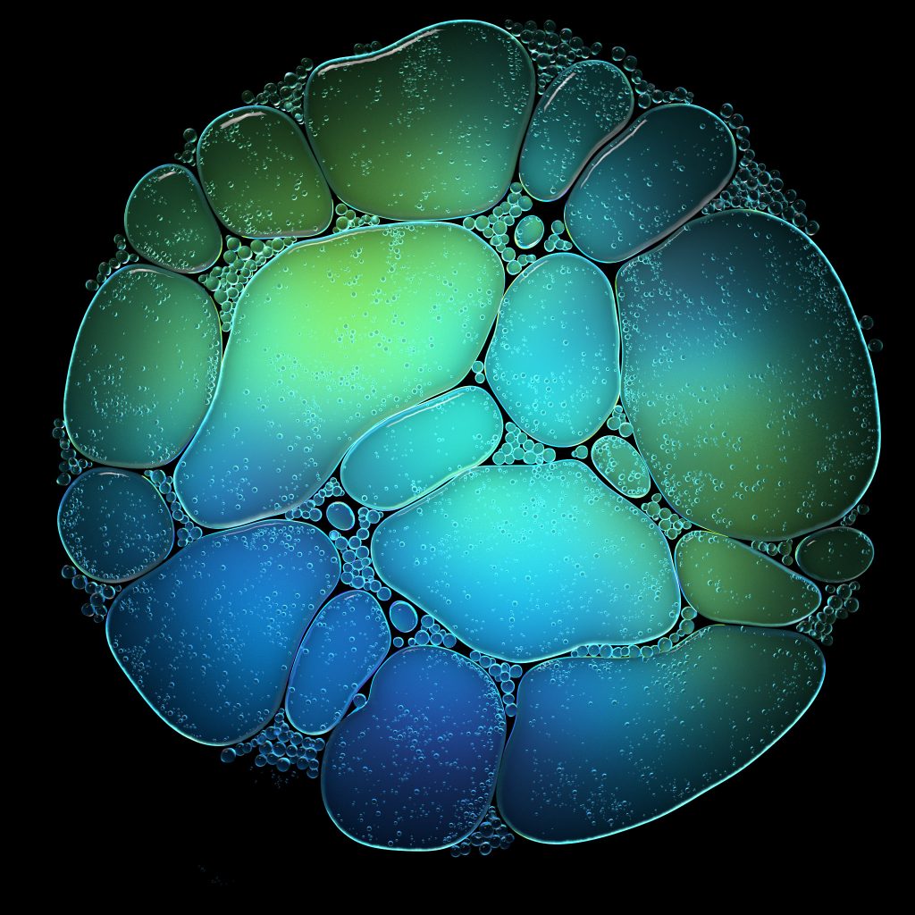
And here’s the final result:
Primary Bubbles Simulation
The first order of business was to get the initial bubble arrangement. The whole primary simulation, including this run-up process, happens in /obj/bubbles_primary_simulation. I scattered a few random points in a plane and copied circles to those points, then jittered them slightly to make the outlines irregular. I also created a circular collision field to contain them during the expansion process. The expansion itself was achieved by turning the circles into Vellum Hair, and then slowly scaling up the f@restlength attribute of the hair constraint primitives during the simulation. In this first stage I used two SOP Solvers to handle this expansion, although it’s generally faster to use Geometry Wrangles for this (and in later stages I use Geometry Wrangles). One SOP Solver modifies the Geometry simulation data, which is the default data to edit, and this Solver simply forces @P.y to remain at zero, keeping the expansion completely flat. The other SOP Solver is applied to the ConstraintGeometry data, which is the simulation data that contains the constraint primitives. This Solver multiplies the constraint primitives’ f@restlength attribute by a very small amount (1.004) each timestep, resulting in a slow expansion over time. A Switch turns off this expansion after frame 50 so that the simulation can stabilize. The high drag value of the constraints allows this to happen without too much jittering. Here’s what this expansion looks like:
If you haven’t dealt with the “data” members of DOP objects before, jump inside the dopnet1 DOP Network and take a look at the Geometry Spreadsheet. If you expand vellumobject1, you’ll notice a list of properties with names like “Basic”, “Options”, “RelInAffectors” and the like, and then a few objects with a cube icon next to them. These objects are SOP data that can be modified by a SOP Solver (or a Geometry wrangle). If you want to modify data other than the default “Geometry”, you just need to change the SOP Solver’s “Data Name” parameter to match that data name. So if you want to manipulate constraints in Vellum during the simulation, all you have to do is change the “Data Name” to “ConstraintGeometry”.
A quick note: you can also import more than one of these data points into a single SOP Solver if you like; you can only write to one of them, however. Just duplicate the “dop_geometry” node that comes built into the SOP Solver, and change the “Geometry Data Path” parameter to be whatever geometry data name you want to grab.
I just ran this simulation until it settled down, then used a locked Timeshift SOP to cache it in-place. The next step was to handle the smaller bubbles that are trapped in the gaps between the larger ones. To determine the starting locations for these bubbles, I made a large circle representing the circular collision field and extruded it into a volume, then did the same to the large bubbles. Subtracting the large bubble volume from the circular volume leaves the negative space in between the large bubbles, which is then run through a Volume Slice (again to keep things in 2D for now) and then points are scattered on this flat plane. After a Relax operation to keep the bubbles separated, any points that have been pushed out of the safe area are flagged (via the flag_overlaps Wrangle that samples the original scatter volume) and later deleted. These remaining points will be simulated as Vellum Grains, and for visibility a Sprite SOP is used to display them as spheres.
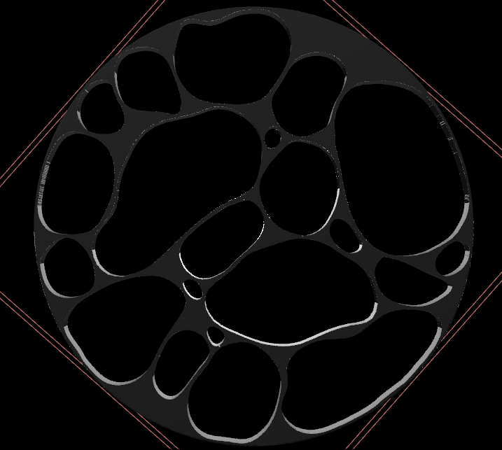
The SDF volume representing the negative space between the large bubbles. 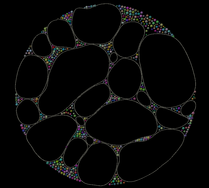
The sprites representing the small bubbles, after relaxation.
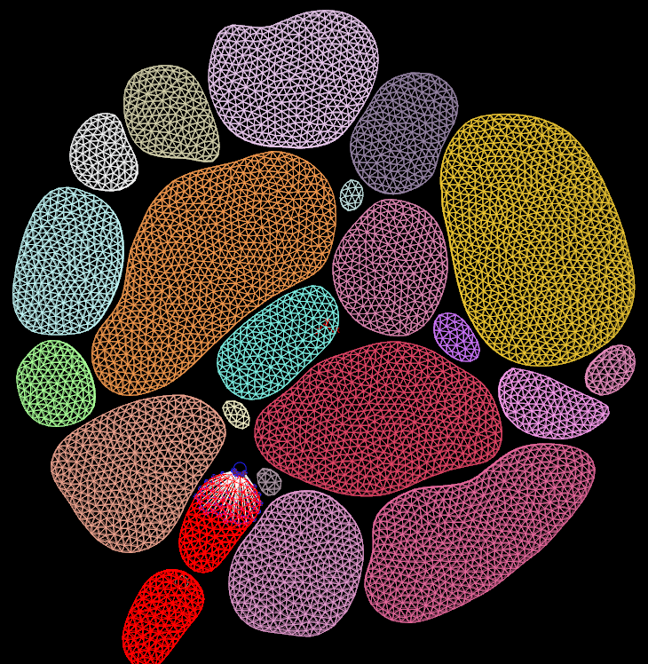
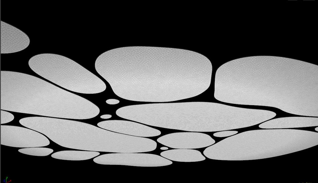
Now, a little prep work before the big simulation. A specific large bubble is chosen for the “animation” group; we’ll use this later as the main bubble that’s dragged through the scene. It’s flagged with a bright red color for visibility. Next, the large and small bubbles are split off so that they can each be configured separately. The large bubbles are run through the new Planar Patch from Curves SOP, which turns them into triangulated planar geometry. The small bubbles are just merged back in after a Switch named “TEST_MODE”… this is just so that I could fine-tune the simulation parameters for the large bubbles before adding in the small ones, which required significantly more substeps and thus took a lot longer to simulate properly. Another Split precedes the main part of the Vellum configuration. First, the “animation” bubble is duplicated and its group is renamed “filler”… this is the bubble that will move in and close the gap behind the “animation” bubble so that the remaining bubbles stay tightly packed.
The large bubbles are then extruded and run through a Vellum Configure Tetrahedral Softbody constraint. In my original experiments here, I tried to keep the simulation entirely 2D by using a SOP Solver to force the Geometry and ConstraintGeometry to stay in the XZ plane (as with the run-up simulation). However, in practice, getting this simulation to be stable required way more substeps than it was worth, especially once the small bubbles (as Vellum Grains) started to get merged in. The Tetrahedral Softbody method required that the objects had some thickness, and this introduced some complications later on, but it made this simulation a lot more bearable to iterate on.
A Circle SOP and two animated Transform SOPs are the drivers of the primary motion here. One Transform controls the “animation” bubble, and the other controls the “filler” bubble, by way of the Vellum Attach to Geometry constraint. The bubbles are simply dragged through the other bubbles, using very stiff (and slightly dampened) constraints between the Circle and the bubble points.
The smaller bubbles are a simpler process; I prune some bubbles that are just a little too close to the large bubble geometry before simulation, and then manually (via a Point Wrangle) create the attributes necessary for simulating the small bubbles as grains: i@isgrain (set to 1), and f@mass.
The only other thing going into this next DOPnet is a simple collision volume shaped like a sandwich. This was necessary after changing the sim from fully 2D to a sort of 2.5D with the Tetrahedral constraints… I still needed the bubbles to mostly act as if they were flat, so the colliders were used to keep them within a narrow vertical range without crushing them completely.
After all this setup, the simulation is really simple. The settings on the Vellum Solver took some fussing over, and the exact animation of the bubbles needed to be adjusted several times in order to have them carve a path through the others that didn’t result in them completely overlapping other bubbles or trapping them in weird ways, but otherwise the only interesting thing in the whole DOPnet is the “force_inwards” POP Wrangle. (POP Wrangles act on the points of Geometry data in your simulation, and this means you can use POP Wrangles on Vellum geometry as well as Packed RBD geometry if you like.)
The very last step here is to take the simulated tetrahedrons, and use them to deform the original polygon geometry. I wasn’t using any embedded geometry here like you would with FEM, so I had to do this manually (there’s probably a better way?). You’ll notice that even though the cached result of the simulation and the original extruded geometry look the same, one of them is comprised of polygons, and the other of tetrahedrons. I wanted nice clean polygons for the next step. In order to keep each simulated bubble deforming only the bubble it matched, I used the i@class attribute, generated earlier via a Connectivity SOP, to add to the @P.y attribute for both the simulated geometry and the original static geometry. I then ran a Point Deform SOP, and afterwards reversed the addition to @P.y. There are likely more precise ways to keep different objects from influencing each other during a Point Deform, but this is pretty easy to set up and executes quickly.
Bubbles Post-Simulation
There’s a brief post-simulation step here, after the clean deforming geometry is generated. You’ll notice that the timing of the above GIF is a bit… mushy. There’s also some rather jittery points in there, especially in the Vellum Grains. The jittering is easily addressed using a Filter CHOP… a slight temporal blur applied to the point positions makes the popping and jittering look a little more natural (too much can mess up the animation, though!). The mushy movement at this step is somewhat on purpose. Vellum is pretty sensitive to fast movements, and in order to avoid excessive substepping and also have some flex room at this post-simulation step, the animation is intentionally a bit slow. After filtering, I used a Retime SOP to add some more “snap” to the movements, so that the bubble accelerates much more quickly and eases into its end position. I also added a very slight amount of rotation to the geometry as a whole after it settles, to keep things from looking too static at the end.
Secondary Bubbles (Fizz) Simulation
A lot of the visual interest here comes from the swirly little “fizz” particles moving inside the larger bubbles. Generally when you see “swirly” motion in CG, the first thing you should be thinking of is “fluid simulation”, because the swirly, vortex-like movement you see in both liquids and smoke are caused by the same underlying principle: incompressible flow. If you assume that your medium, be it air or water, is more or less incompressible, the equations for handling fluid velocities become much easier than they otherwise would be, and in computer graphics we like things to be easy, so liquid and gas simulations generally make this assumption. If two jets of gas or water are pushing towards each other, the solver will try to compute a velocity field that adjusts the competing velocities such that they push around each other rather than canceling each other out, forming swirls. In Houdini this is caused by the Gas Project Non-Divergent microsolver that exists inside both the Smoke Solver and the FLIP Solver.
Okay, nerd stuff aside, what this means for this simulation is that I handled it using 2D Smoke, which is about as cheap as it gets when it comes to fluid simulations. First, the initial state of the fizz is generated. I just convert the bubbles into a VDB Volume, multiply the density volume by some procedural noise in a Volume VOP, then scatter points within that density. The Volume Slice is used both to visualize this density, and as a surface to project the points onto when running them through the Relax SOP after randomizing their @pscale attribute a bit for variation. Copying sphere primitives to those points for visualization is the last step; now onto the fun stuff.
Generating the Velocity Field
This first part of the network is a bit ugly, but it’s not too bad. There are four different inputs to the velocity volume simulation secondary_bubble_volumes:
- POINT_VISUALIZATION: Just the input points themselves, for use with the Static Object DOP. These are only to see the geometry moving inside the DOPnet, to make sure the volumes are colliding correctly.
- VELOCITY_SOURCE: Here I’m just computing the velocity of the source points, then rasterizing those points into a velocity field. The upstream Copy SOP is just to sort of artificially “thicken” the velocity field, because I was having some issues sampling it when it was flatter.
- INVERSE_COLLISION_VOLUME: This is an SDF volume that’s inverted so that the “insides” of the bubbles are now facing in the other direction. This way the fizz bubbles will stay inside the collision volume rather than being pushed outside.
- DENSITY_VOLUME: This isn’t entirely necessary but it makes the volume motion much easier to understand. I’m just randomly scattering density around, for the initial state of the volume that’s going to be pushed around by the bubble movement.
The inside of this DOPnet couldn’t be simpler. The Static Object DOP sources in the POINT_VISUALIZATION as the SOP Path, so that the original bubble motion can be shown. This geometry isn’t used to create the collision volume, though; instead, the Mode of this DOP is set to “Volume Sample” and the Proxy Volume parameter is set to point to the INVERSE_COLLISION_VOLUME generated in SOPs. The Static Object DOP tends to make really slow and clunky collision volumes, so this workflow means that all the nifty VDB tools can be used to quickly generate (and cache!) collision volumes to speed up simulation.
The Smoke Object is using DENSITY_VOLUME as its Density SOP Path under Initial Data, and isn’t really changed from there. Running the simulation as Two-Dimensional means it will simulate very, very quickly. Again, this is just to make it easier to see what the volume is doing; the density field isn’t used for anything else.
The Volume Source DOP sources in the VELOCITY_SOURCE’s vel field in “pull” mode, which tries to blend in the source velocity from SOPs anytime it’s accelerating the existing velocity, and ignores it when it’s slowing down. This means that the simulated velocity field will speed up to match what the animated bubbles are doing as quickly as possible, but the field won’t slow down when the animation stops, leaving plenty of time for the swirling to continue on.
Advecting the Fizz
This part is really easy. The fizz points, velocity field, and collision field are already generated, so the only thing left to do is advect the particles through the velocity field. The particles are given POP Grains attributes (and Assume Uniform Radius is disabled since the particles are all different sizes), they’re pushed through the velocity field using POP Advect by Volumes, a little drag is applied, and then the bubbles are forced to stay on the XZ plane via a POP Wrangle (still trying to stay in 2D here!). The same collision volume from before is used to contain the particles so they can’t escape the boundaries of the larger bubbles.
Meshing the Bubbles
This part proved trickier than I’d expected. The planar patches that make up the bubbles had the right motion on a flat plane, but in order to render like bubbles, they need to be smoothed out quite a bit, and this took a few steps to figure out.
First, these buttons were flattened by deleting the extruded parts and setting @P.y to zero. I output the flattened bubbles, along with their “resting” position via a Time Shift, to a couple of nulls for use later on when Point Deforming. Next, the flattened planar patches had their inside polygons removed and resampled, smoothing out the borders of the bubbles to make them look more acceptably liquid.
The big For/Each loop in the middle figures out how much each of these bubbles will be extruded. The insides of the bubbles are regenerated in a static pose (matching the “resting” position we defined earlier) at a much higher resolution than before, and the edges are grouped. A Falloff SOP computes the geodesic distance between the edges of each individual bubble and each point within that bubble, kind of a signed distance field. That value is blurred via an Attribute Blur, and then the minimum and maximum for each bubble is computed before mapping the final falloff value to a ramp parameter, using the minimum and maximum as bounds. This falloff value is going to be used to extrude the bubbles, with the Falloff Ramp parameter on the last Point Wrangle defining the “silhouette” of each bubble.
After the loop, the “dome_bottom” and “dome_top” Point Wrangles push the back side and front sides of the bubbles outwards, according to the falloff attribute. This bulge will help sculpt the reflections and refractions of the bubbles, to keep the insides a little more interesting.
The flat bubbles, viewed from a side angle. 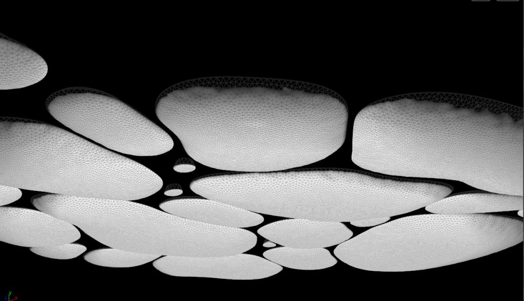
The extruded bubbles with the bulge applied based on the “falloff” attribute.
The same Point Deform trick that I used earlier on in the process is used here to move the bubbles apart from each other in space using the i@class attribute, so that the neighboring bubbles don’t interfere with each others’ deformations. Point velocity is re-computed after the Point Deform in order to allow for motion blur. An important bit of processing here that I didn’t realize I needed until rendering was to blur out the N attribute quite a bit. You can see in the above-right picture that the geometry is a bit wrinkly. This was unavoidable even with very high subdivisions… likely an artifact of using geodesic distance to generate the falloff attribute that creates the bulge. Blurring the normals makes the reflections and refractions appear smooth in rendering despite the slight irregularities in the surface.
The small bubbles don’t need much special treatment; a polygon sphere is copied to each point and then slightly deformed with some sparse convolution noise in a Point Wrangle, to make them appear a little bit irregular. They’re merged back in with the regular bubbles.
Meshing the Fizz
This was probably more complicated than it needed to be, but such is the nature of effects work. I wanted the fizz to appear to have some depth despite being solved entirely in 2D, so I used a bit of VEX to randomly jitter @P.y on the fizz points. However, the bubble heights aren’t consistent at all, so to keep the fizz inside the bubbles, I needed to create a sort of collision volume out of the large bubbles to contain them. After converting the bubbles to VDB SDFs and caching them, I used a little VEX to keep the bubbles inside the surface:
float sample = volumesample(1, 0, @P);
vector grad = volumegradient(1, 0, @P);
if(sample > 0) {
    @P -= (grad * sample + (@pscale/2));
}
This was all well and good on static frames, but of course this procedural solution introduced jittering when moving from one frame to the next. The quick-and-dirty solution (my favorite!) to this problem was to simply filter the point positions after running this simple collision effect, via a Filter CHOP just like before. After recomputing the velocities, these points were cached, and small polygon spheres were copied to the points.
Lighting and Rendering
This part was really tricky to get right. Refractive surfaces are always annoying, and this image was nothing but. Redshift, my current favorite render engine, is thankfully quite snappy when set up correctly, so I could at least iterate quickly.
Early tests were not very promising:
There’s a lot wrong here, but much of it was because of the lighting setup itself, not the materials in particular. Aside from the ugliness of the photo plate used and the lack of color contrast, the edges of the bubbles were too sharp and the edge refractions seemed too angular.
I took a step back and looked at some examples of how people tend to photograph bubbles in the real world. Many of these examples were all about photographing the reflections of the diffractive thin layer, similar to what Apple used for the iPhone X, which gets you all kinds of wild colors but not the transparent refractive effect I was going for. After digging around through Google Images for a while, I found this image from a photographer’s website, along with some shooting hints:

I switched my background plate to a colorful procedural noise pattern, and adjusted the lighting setup so that it was entirely backlit. The background plate was given a translucent material so that it could transmit light through the bubble refractions. The result looked like this:
I messed around with the lighting for what felt like ages, trying to get the right amount of light through so that the bubbles felt translucent. At one point I tried changing the backplate from a flat geometry to a bowl shape, and then rendered an image that was far too overexposed and white, but the details on the edges of the bubbles was perfect. It turned out that the bowl shape had pushed the backplate beneath the area light underneath the bubbles, so I wasn’t using the backplate at all. Duh. I hid the backplate and assigned the procedural color texture to the light itself, and got this:
I hope this breakdown was useful for you! I wouldn’t want to let anyone down by not providing the .HIP file, so here it is, with some caveats:
- Some things might not work perfectly, and if they don’t, please contact me. This project evolved organically so some pieces may not be left exactly as intended.
- None of the solutions I’ve mentioned above are the “best” solutions. In fact, many of them are probably dumb or inefficient. If you see anything here that can be done better, please tell me!
Anyways, here’s the HIP, and enjoy!
25 Comments
Patrick Krebs · 11/23/2019 at 12:26
You’re a genius. I can’t wait to replicate this over my Thanksgiving break. I’ll let you know how it goes!
vincent · 12/29/2019 at 15:42
Awesome tutorial, thanks you so much, you such a smart mind!
Denis Jagodic · 05/04/2020 at 14:13
Dear Henry, i am amazed and terrified at the same time. You are a genius, no doubt! Your blog is a blessing and you motivate me ALOT. I hope that someday i’ll achieve as high fidelity thought processes as you. Keep on going! Thank you for sharing all of this! <3
toadstorm · 05/04/2020 at 14:21
I really appreciate it! I don’t want anyone to mistake me for a genius, though, it’s just a lot of long years working at these concepts. I’m very happy to hear my blog has been helpful for you!
vincent thomas · 07/09/2020 at 11:22
Your breakdown and tutorials are the cream of the cream. You are smart and highly skilled, thanks you for sharing with us your research
toadstorm · 07/09/2020 at 11:25
Thanks so much, and I’m happy to share!
ky duyen · 06/26/2021 at 07:20
can you repost the hip file? I can’t seem to download it. Thank you
toadstorm · 06/26/2021 at 08:34
I just checked the link, and it seems to be working here. Try again?
John · 08/16/2021 at 18:02
The link wasn’t working for me, but when I copied it and pasted it in a new tab I was able to download the file. ¯\_(ツ)_/¯
Tuber · 01/25/2022 at 10:06
Great lesson, thanks, but the link is not working ((((
toadstorm · 01/25/2022 at 10:20
Looks like it was an HTTPS error, sorry about that! Should be working now.
doyaooi · 03/04/2022 at 05:34
Thank you very much for your help,I’m a new learner,I’m having some problems with your project,Inside the bubbles_primary_simulation node ,Dopnet3 is unresponsive in this simulation,I just can’t find a solution,Can you suggest a solution? Thank you very much…
toadstorm · 03/04/2022 at 09:36
I’ve noticed this happening with other files specifically using Vellum simulations. It might be a Houdini bug… you could try updating to a more recent production build of Houdini and see if that works better? Sorry I don’t have a better fix for you!
doyaooi · 03/04/2022 at 21:23
Thank you very much,So far, I’ve tried a lot of things, but nothing,The software is up to date,Could you please provide me with another contact information? I will send you screenshots of the problems I have encountered. Thank you very much.
toadstorm · 03/05/2022 at 01:04
You can contact me at henry@toadstorm.com
Tim · 04/14/2022 at 12:52
I am wondering about the lighting. The backlight has a texture labeled op:/img/light_tex/OUT and I cannot find it. Is that the “procedural color texture” and must be built. Sorry, I am still learning Redshift in may ways.
toadstorm · 04/14/2022 at 12:56
The texture exists as a procedural in /img/light_tex/OUT. You’re saying you can’t find that node in the posted scene? The prefix op: means that the texture is not a file and needs to be cooked.
Tim · 04/14/2022 at 21:04
I see, that makes sense. I thought it was a file. I get it. I think like others I have some issues with the hip. the constraints stop working from section one when I cached. I am reloading it because the time shift is set anyways but I wonder why that happened. Such an amazing set up to learn from.
TIm · 04/14/2022 at 23:08
I ran into the same situation with Dopnet 3 in bubbles_primary_simulation, albeit is says that “The number of points in the geometry and constraints do not match.” I’ve seen other bugs from H19 updates. That is what I mean about running into issues with the hip file. Anyways, it is really crazy you were able to work this all out. Thanks for posting this.
toadstorm · 04/14/2022 at 23:12
I haven’t tried sorting through this project in Houdini 19… I get the feeling a lot of subtle things about Vellum have changed since I wrote this article. If it’s a quick fix, I’ll upload a new version, but I need to step through and see how badly this file gets mangled by the update.
Tim · 04/14/2022 at 23:53
I suspect that is right. I’ve run into that with a lot of older content. It’s not a big deal as long as I can work out how you did it and I think I think I can. A gleaned a lot of good techniques from this. The lighting from the back was something I hadn’t expected. It looks great and does bring out depth and illustrated how much can be gained from the extra work.
toadstorm · 04/15/2022 at 11:10
I figured out the issue… it was the way in which I was merging in Vellum Grains without constraint data with the Vellum Tetrahedrons geometry. It was possible in Houdini 17.5, but not in 19.0. I switched to using Vellum Pack on both streams, then merging, then unpacking before simulation.
I’ve updated the .ZIP file in this post to account for this change. It should work fine now. Please let me know if it doesn’t!
Tim · 05/24/2023 at 11:36
I love coming back to this after a year or so in Houdini because it really illustrates how much I did not know, how brilliant this piece really is, and how well this breakdown is formatted. This is and always will be one of my favorite Houdini Projects.
Obagi · 04/14/2025 at 10:24
I encountered the same problem in version 20.0, and I spent a whole night to find out where the problem was. In the advanced tab of the new version of vellum solver, the “assume uniform radius under grain collision” option is turned on by default. Turning it off can solve the error “the number of points in the geometry and constraints do not match”. Finally, thank you for sharing everything, it is still helpful in 2025 :)
olivier · 10/03/2025 at 04:49
thank you very much for sharing !