Revisiting Parallel Transport

I was asked the other day about fixing a little issue with MOPs Orient Curve, a node that really hasn’t changed much in MOPs since it was first launched way back in 2018. Most of the reason it hasn’t been revisited is because a few versions ago SideFX created their own curve orientation tool, the aptly-named Orientation Along Curve SOP, which more or less does what MOPs Orient Curve did but with more technical options.

However, the user was having trouble getting Orientation Along Curve to do exactly what he wanted and I figured I’d take a second look at the MOPs tool as it was one that was originally written by Manu from Entagma, using the Parallel Transport method outlined in his handy VEX tutorial. I never had to get too involved in this part of the toolkit because Manu already handled all the math for me, so this was a perfectly good excuse for me to learn the algorithm and see if I could improve the functionality a bit. Hopefully this is also a good look at how this algorithm works for the reader who doesn’t want to watch an eight-year-old Vimeo tutorial.

First, the source issue: on a closed circle, why do the end points at the 3 o’clock position here have slightly skewed orientations?

The problem is grounded in the fact that the 3 o’clock position on this particular circle are where the first and last points on the circle primitive meet. Manu’s original implementation of the parallel transport algorithm, based on this paper here, starts on the first point of the curve and computes orientations from first point to last point. Each point is figuring out what its tangent vector is (what direction points to the next location on the curve) based on the position of the next point in line. If there’s no more points in line, though, the algorithm just extrapolates the next tangent based on what the previous one looked like. It wasn’t really meant for this edge case where the start and end points are linked!

What’s parallel transport?

Let’s take a step back and talk about what this algorithm even does. If you read the linked white paper it looks like a bunch of insane wizardry because, like all good white papers, the math has to be done with proofs, and if you’re not used to reading those it looks like absolute hell. However the idea behind it and the implementation of it, when done on discrete sets of points like what you deal with in 3D graphics, is really not terribly complicated.

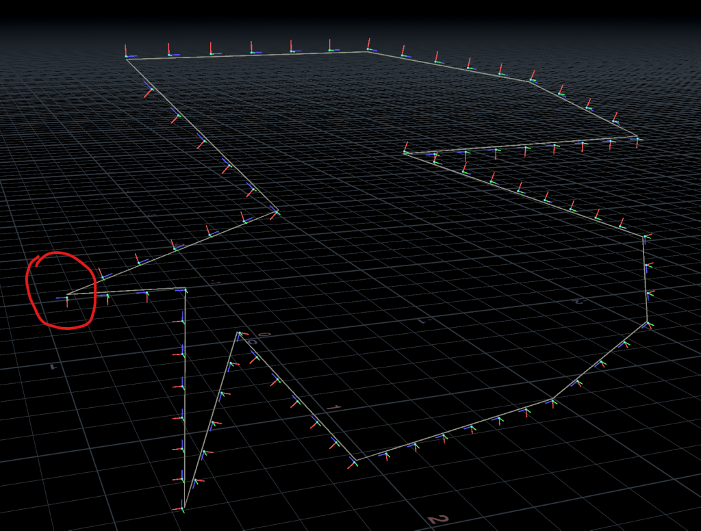
The goal of parallel transport is to create a smoothly-transitioning orientation along a set of edges so that you don’t end up with sudden flips or discontinuities along the line. If you’ve ever tried to animate something along a path or copy objects to the points of paths with lots of twists and turns, you’ve likely seen this problem before. Here’s a loopy curve with an orientation created by the very naive Polyframe SOP that just guesses at orientations based on computed tangent and normal vectors:

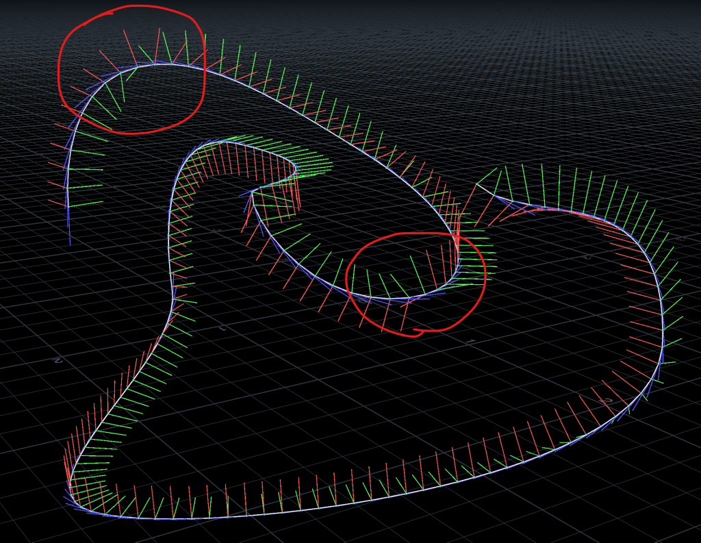
You can see in those circled areas that there are sudden flips in the green and red vectors. This happens in part because each point on the curve is more or less computing its local tangent (blue) and normal (green) vectors independently of any other location on the curve; they just look at their immediate neighbors and figure that’s good enough.

Now the same curve orientations computed via parallel transport:

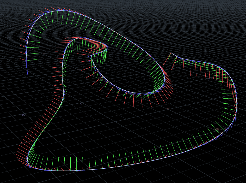
The core idea here is simple: starting at the beginning of the curve, get the tangent to the curve and a normal vector. Then for each successive point along the curve, figure out the angle that would rotate the previous tangent vector to match the next tangent. Then rotate the normal vector by that same angle, around the binormal (the red vector in the above images). The binormal is a fancy way of saying a vector that’s orthogonal to the tangent and normal vectors, meaning it’s an axis perpendicular to both those other vectors.

If you’ve ever read my Even Longer-Winded Guide to Houdini Instancing you might remember that in order to compute an orientation you need to have three vectors: a “forward” direction, an “up” direction, and a “side” direction. The “side” direction, however, can be automatically computed by determining the cross product of the other two vectors. Crossing two vectors gets you a third vector orthogonal to the other two. In parallel transport we’re doing the same thing to get the binormal vector that we use as the axis of rotation for our normal vectors.

By incrementally applying these small rotations to the normal vectors along the length of the curve, the algorithm ensures that there’s no sudden flips or discontinuities in orientations while passing along the curve, regardless of how many twists and turns are present. Conceptually it’s not too bad! The implementation is, as always, the annoying part.

Computing Tangents

The first thing to do to make this algorithm work is to compute the tangents along the curve. In Manu’s original implementation for MOPs, the tangents were always computed by starting at point i, looking ahead to point i+1, subtracting their point positions from each other, and normalizing the result. This gets you a vector pointing to the next point along the curve. This was the original VEX code:

for (int i = 0; i<pntcnt-1; i++)
{
push(tangents, normalize(point(geoself(), "P", pnts[i+1]) - point(geoself(), "P", pnts[i])));
}

However, as we saw in the first illustration, this fails when you have curves that join at the ends. It also tends to run into trouble when you have curves with sharp corners; those abrupt changes in direction can mean anything you copy to those points or slide along them will have similarly sudden changes in orientation you don’t want. So what to do?

Rather than using point numbers to determine the next point along the line, we can instead use vertex connectivity. We can see that the first and last points on the curve are joined together as part of a single polyline primitive, but points alone don’t have this connectivity information. Vertices do!

One of the extremely cool things about Houdini is that so much of the various contexts use points and vertices to describe things beyond just geometry. Rigid body and Vellum constraints are two-vertex primitives connected together with a single polyline primitive. APEX graphs are just geometry, with points describing functions and parameters and vertex connectivity describing inputs and outputs to these functions, like a node graph. Most importantly for us, the KineFX rigging system also uses vertex connectivity to define parent/child relationships between joints. This means we can lean on the KineFX helper functions in VEX to quickly and easily determine both the next and previous points of each point along the line, without getting in the weeds with pointvertex() or pointhedge() or anything else. It takes a certain kind of sick person to actively want to do anything with half-edges and I figure most of my readers here would rather find an easier route.

The library in question we want is the KineFX helper library for rig hierarchies, called kinefx_hierarchy.h. It lives alongside a bunch of other KineFX-related libraries (totally worth checking out) in $HFS/packages/kinefx/vex/include/. If you open it up in a text editor, you’ll see a couple of important functions here, namely getparent() and getchildren(). These two functions crawl along half-edges, using the connectivity of polyline vertices to determine the previous (parent) and next (child) points on the curve. So anyways let’s steal them! All you have to do is start your Primitive Wrangle (because we’re iterating over points in a primitive, in order of points) with this line:

#include <kinefx_hierarchy.h>

You can do this with other built-in VEX libraries, too. It’s worth spending some time checking these out and studying them if you’re reasonably comfortable with VEX.

Forward Tangents

Now we want to compute the tangents for each point along the curve, using the getchildren() helper function. The first point in the array returned by getchildren() is the nearest connected downstream point. We’ll set this up in a Primitive Wrangle so that it operates in the order of points on the curve:

#include <kinefx_hierarchy.h>
int pts[] = primpoints(0, @primnum); 
vector tangents[];
vector normals[];
vector first_normal = point(0, "N", pts[0]);

for(int i=0; i<len(pts); i++) {
    // FORWARD TANGENTS
    int desc[] = getchildren(0, pts[i]);
    int child = desc[0];
    if(len(desc) > 0) {
        // tangent is child's position minus mine
        vector P1 = point(0, "P", pts[i]);
        vector P2 = point(0, "P", child);
        vector tangent = normalize(P2 - P1);
        push(tangents, tangent);
    } else {
        // no children found, duplicate previous tangent
        push(tangents, tangents[-1]);
    }
    // add default normal to populate normals array
    push(normals, first_normal);
}

What we’re doing here is creating two empty arrays, one for tangents and one for normals (since we need both to compute the final orientations), and then populating those arrays one at a time with the tangents of the curve and with the first normal found on the curve. The first normal is our starting point for all other rotations; we’ll be overwriting all of the other normals later on. To get the tangents, we get the first point number returned by getchildren(), get the position P of that point, and subtract the position of the current point from that point. Normalizing the result gets us a vector that points straight down the curve to the next point in line. If the length of the array returned by getchildren() is zero, then the point has no children and we just use the last index of the tangents array and copy it (index -1 is Python-like array syntax for “get the last index”).

Backward Tangents

We could also go in the other direction… compute the tangents by looking backwards to the parent point. On some curves this might be preferable to looking forwards! The code is very similar, we’re just relying on getparent() rather than getchildren():

for(int i=0; i<len(pts); i++) {
    // BACKWARD TANGENTS
    int parent = getparent(0, pts[i]);
    // tangent is parent's position minus mine
    if(parent > -1) {
        vector P1 = point(0, "P", pts[i]);
        vector P2 = point(0, "P", parent);
        vector tangent = normalize(P2 - P1);
        push(tangents, tangent);
        push(normals, first_normal);
    } else {
        // there's no parent, so we must be the first.
        // look ahead to the next point, but reverse the result
        // so we're still pointing in the same direction we expect.
        vector P1 = point(0, "P", pts[i]);
        vector P2 = point(0, "P", pts[i+1]);
        vector tangent = normalize(P1 - P2);
        push(tangents, tangent);
        push(normals, first_normal);
    }
}

If you look at the definition of getparent(), it returns -1 if there’s no parent found. If a point has no parent, we can safely assume it’s the start of the curve, so we just look to the next point in line to get the tangent vector and then reverse it so it’s pointing in the same overall direction as the other tangents will be.

Averaging Tangents

A third option would be to get the average of both neighboring tangents. We can look ahead for the forward tangent, look backwards for the backward tangent, flip one of them, then average them both together to get a blended result. For curves with sharp corners like the above example, this can sometimes get us smoother results. Check it out:

 for(int i=0; i<len(pts); i++) {
        // AVERAGE OF BOTH TANGENTS
        int desc[] = getchildren(0, pts[i]);
        int child = desc[0];
        int parent = getparent(0, pts[i]);
        
        vector P1 = point(0, "P", pts[i]);
        vector P2 = point(0, "P", child);
        vector P3 = point(0, "P", parent);
        
        // average between forward and (flipped) backward tangents
        vector tangent1 = normalize(P2 - P1);
        vector tangent2 = normalize(P3 - P1) * -1;
        
        // exceptions for start and end points
        if(len(desc) == 0) {
            tangent1 = tangents[-1];
        }
        if(parent == -1) {
            tangent2 = tangent1;
        }

        // blend forward and backward tangents
        vector tangent = normalize(lerp(tangent1, tangent2, 0.5));
        
        push(tangents, tangent);
        push(normals, first_normal);
    }

Tangents Comparison

We’re getting ahead of ourselves a bit here but it’s helpful to see a visual comparison of these different approaches to computing tangents:

As an aside, notice how the tangent of the point all the way on the far left (the one that was circled before) isn’t pointing out into space anymore? This is because of our new approach to getting tangents based on connectivity instead of point number! We still have to actually implement the algorithm, though…

Computing Normals

Now that we have the tangents figured out and added to an array, it’s time to actually calculate the normals. If you look at page 9 of the white paper, you’ll see this extremely helpful (but somewhat confusing) pseudo-code for the algorithm:

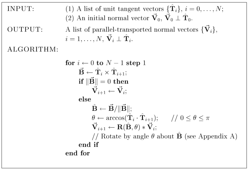
Translating this into something a little more human-readable:

• For each point of the curve (except the last one):
  • Compute the binormal by cross multiplying this point’s and the next point’s tangents
  • If the binormal is 0, this means the tangents are parallel and we can set the next point’s normal V to be the same as the current point’s normal.
  • If not, first normalize the binormal (divide it by its own length).
  • Next, a little trigonometry: compute the angle that would rotate this point’s tangent to match the next point’s tangent.
  • Rotate the next point’s normal vector around the binormal, by the computed angle.
  • Store the next point’s updated normal vector and continue on.

An interesting quirk here that will come up later when we code this, and one of the reasons we’re doing everything via temporary arrays instead of binding things to attributes like we often would in wrangles, is that we’re setting the values of the next normal in line (index i+1) and not the current index!

The trigonometry bit (sorry)

Those of you with a mediocre math education like mine (thanks America) are probably going to be a bit put off by that bit of arccos magic that’s happening in the algorithm. In short, you can find the angle between two unit vectors by computing the arc cosine of the dot product of the two vectors. Let’s take a step back and break down what that means.

Dot Product

The dot product of two vectors can be used for a lot of things, but in short it’s a measurement of the similarity of two vectors. If the dot product of two normalized vectors (meaning the length is 1.0) is 1.0, they are parallel. If the dot product is 0.0, they are orthogonal (perpendicular). You can think of it like a kind of ratio between two vectors.

Arc Cosine

If you remember SOHCAHTOA from trigonometry class, you might remember what the cosine of a triangle is. The cosine is a measurement of the ratio (there’s that word again) between the adjacent side of a right triangle and the hypotenuse side, relative to a given angle. It’s easier to see this as an illustration:

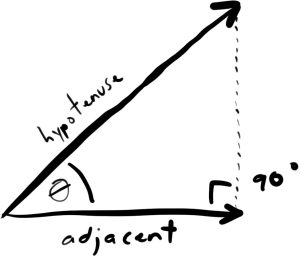
The cosine of the angle Ɵ here will be equal to the ratio of these two sides of the triangle, whatever they are.

Now imagine that these two sides are your two tangent vectors, superimposed onto each other. You know that the cosine of the angle between these two vectors will be equal to the ratio between them. You now know that ratio, because it’s the dot product! Take a look at this identity:

cos(Ɵ) = dot(v1, v2)

The only question, then, is how to get that angle Ɵ given the dot product you have. The answer is the inverse cosine, often called the arc cosine. This lets you get that angle based on the ratio you have:

acos(dot(v1, v2)) = Ɵ 

Now you have the angle between the two tangents and you’re ready to transform the normal vector!

Rotating the Normals

Now that we have all our tangents computed and we understand how to calculate the angle between one tangent vector and the next, we can finally use this information to rotate each normal vector by this same angle, one at a time along the curve points. For each point in the array (except the last one), we’ll compute the binormal between the current tangent and the next, compute the angle between the same, and then rotate the normal around the binormal by that angle. Compare this to the human-readable series of steps above:

for(int i=0; i<len(normals)-1; i++) {
    // get a vector orthogonal to the current and next tangent. this is our
    // axis of rotation for rotating the normal.
    vector binormal = cross(tangents[i], tangents[i+1]);
    // if the two tangents we're testing are parallel, crossing them will return
    // a zero-length vector. we can skip the rest of this math and just assume the
    // orientation hasn't changed.
    if(length2(binormal) == 0) {
        normals[i+1] = normals[i];
    } else {
        binormal = normalize(binormal);
        // find the angle that rotates this tangent onto the next
        float theta = acos(dot(tangents[i], tangents[i+1]));
        // rotate the current normal around the binormal by this angle
        matrix3 m = ident();
        rotate(m, theta, binormal);
        // rotate the next normal by this amount and set it
        normals[i+1] = m * normals[i];
    }
}

The only thing we haven’t really talked about yet is that matrix3 and rotate() function in there. Again going back to the Even Longer-Winded Guide to Houdini Instancing, if you want to transform a vector (meaning rotate, translate, or scale), you can multiply it by a matrix. In this particular case we only care about rotation, so instead of a full 4×4 matrix we’re using a 3×3 matrix3 to handle the vector rotation.

First we create an “identity” matrix, which is like a null matrix that doesn’t do anything. Then we rotate that matrix around the binormal by the angle that we calculated using our fancy arc cosine operation. Then we multiply our current normal by this matrix to rotate it, and apply the result to the next normal in the array (again, index i+1).

Binding the Result

These arrays are done but we still have to actually create Houdini attributes out of them. There are a lot of different ways you can store orientation data in Houdini, but my preference is to use the orient attribute, which is a vector4 (four numbers) stored as a quaternion, a kind of math wizard shorthand for rotations that I can’t possibly explain here. Fortunately VEX will do this all for you. All you have to do is make a transform out of the tangent and normal vectors we have in our array, and then let VEX convert that to a quaternion:

// bind arrays to attributes
for(int i=0; i<len(pts); i++) {
    vector N = normals[i];
    vector T = tangents[i];

    // build orthonormal matrix
    matrix3 m = maketransform(T, N);

    // create quaternion and write to point attribute
    vector4 orient = quaternion(m);
    setpointattrib(0, "orient", pts[i], orient, "set");
}

The reason we have to use setpointattrib() instead of just setting p@orient is because we’re again in a Primitive Wrangle SOP; we’re not operating on points. This is technically a little bit slower than setting point attributes in a Point Wrangle SOP, but because we have to iterate over all the points in order instead of in parallel, we have no choice. The maketransform() function creates a transform matrix out of two vectors: a forward vector and an up vector. For the purposes of orienting things along a curve, I like to use the tangent of the curve as the forward direction, which is why it’s used as the first term of maketransform(). If you prefer objects facing the normals instead you could always swap the terms.

Now with our orient attribute bound we can use MOPs Visualize Frame to see the resulting orientation! Here’s a comparison again of the default orientation created by a Polyframe SOP just dumbly guessing at tangent and normal vectors, and our implementation of Parallel Transport that’s smoothly rotating those orientations from start to end:

Take a close look again especially at the green vectors. Those are the normal vectors that we rotated into position using Parallel Transport. You can see with the default Polyframe orientation method, there are areas where they flip from one side of the curve to another, generally at points of inflection along the curve. Parallel transport makes all the normals nice and consistent along the entire length.

Extra Fixins

You can always add more stuff to this process to make things more useful or predictable. If the first curve normal is too similar to the first tangent, for example, you can’t meaningfully compute a binormal because the vectors are parallel. This often happens on straight vertical lines or circles. In cases like this it helps to have an optional normal override that the user can set before the tangent and normal arrays are filled:

if(chi("override_first_N")) {
    first_normal = normalize(chv("N_override"));
}

In my new implementation for MOPs I’m also including a warning to let the user know if the vectors are too similar so they’re not confused by a bad result:

if(dot(normals[0], tangents[0]) > 0.999999) {
    setdetailattrib(0, "__warning", 1);
}

The Error SOP, when used in an HDA, can output errors or warnings to the user when cooked. In this case I set the “Report This Error” parameter expression to detail(0, "__warning", 0)==1 which evaluates to 1 if the above VEX code determined the vectors are too similar. In the Type Properties dialog of an HDA you have the option to designate Message Nodes; any nodes in this list will have their errors or warnings percolate upwards to the main network view. It’s extremely useful for providing useful feedback to users who might otherwise not know what’s going wrong!

Additionally, you might want to roll, pitch, or yaw the orientations along the length of the curve. This can be fairly easily done by computing more rotations around each axis (roll = Z, yaw = Y, pitch = X) and multiplying the original orientation by these values. Going back again to the Long-Winded Guide, remember that if you want to rotate around a local axis to an existing orientation, you can just rotate a world axis (such as +Z, the roll axis) by the existing orientation to get the axis of rotation you want:

vector twist_axis = qrotate(p@orient, {0,0,1});
vector yaw_axis = qrotate(p@orient, {0,1,0});
vector pitch_axis = qrotate(p@orient, {1,0,0});

Now you can create quaternions representing these additional rotations by providing an angle and an axis as the two parameters to quaternion(). In my example I’m using a @__curveu attribute calculated via a Resample SOP (or a UV Texture SOP set to Arc Length Spline) that gets me the relative position along the curve for each point in a 0-1 range. This neatly maps to ramp attributes so the end user can visually tweak the total amount of rotation along the length of the curve:

float twist_amount = ch("twist_amount") * chramp("twist_ramp", @__curveu);
float yaw_amount = ch("yaw_amount") * chramp("yaw_ramp", @__curveu);
float pitch_amount = ch("pitch_amount") * chramp("pitch_ramp", @__curveu);
vector4 twist = quaternion(radians(twist_amount), twist_axis);
vector4 yaw = quaternion(radians(yaw_amount), yaw_axis);
vector4 pitch = quaternion(radians(pitch_amount), pitch_axis);

Then it’s just a question of what order you decide to combine these rotations in to get the final result. For example here’s applying pitch, yaw, and then roll:

p@orient = qmultiply(pitch, p@orient);
p@orient = qmultiply(yaw, p@orient);
p@orient = qmultiply(roll, p@orient);

Here’s the result of a 720-degree twist around the roll axis, modulated by the position along the curve:

I’ll be including this newer implementation of MOPs Orient Curve in the next Experimental release. Again, this is mostly for educational purposes because SideFX’s Orientation Along Curve SOP already handles this just fine, but it’s never a bad thing to take a closer look at some of these algorithms we take for granted and see what makes them tick. Happy transporting!