I haven’t posted in a long time mostly because I’ve been spending the majority of the last month devouring Houdini tutorials on the internet. Houdini is capable of handling incredibly complex visual effects, and its node-based architecture makes it ideal for effects R&D… if you can get past the learning curve. I’ve never seen a more complicated-looking program.
Anyways, after beating my head against the wall for the better part of a month I’ve finally started making sense out of this program, and I want to share an effect I’ve been researching for an upcoming spot, and turn this into a sort of tutorial for dealing with particle systems, creating objects on the fly, and manipulating shapes using audio. Later on I’ll also go over how to make the effect into a “digital asset,” meaning packaging the effect into a single node with its own interface that you can then use for other shots or share with other artists.
I really dislike video tutorials so I’m going to try to write this one out. The first segment will be about creating the trails, the second will be about modifying the trails using CHOPs, and the third will be about repackaging the effect as a digital asset and building an interface.
Anyways, here’s the effect we’re creating:
I realize it kind of all turns to spaghetti in the end, but that could probably be fixed with a little more fine-tuning, and I wanted to show a little complexity to the effect. Hit the jump for a big huge post about how this is done.
So, how do we make this? I am going to assume you know the very basics of Houdini, like how to make an object and animate it from place to place. If you’re like me and took a really long time to understand all the “OP” lingo, here’s a quick rundown:
- SOP = surface operator (a node relating to geometry, in the “obj” context)
- POP = particle operator (a node relating to a particle network, or POPNet, in the “part” context)
- CHOP = channel operator (a node that modifies channel information such as an animation curve or an audio clip, in the “ch” context)
- ROP = render operator (a node that outputs images, geometry caches, etc, in the “out” context)
There are other OPs (DOPs, VOPs, SHOPs, etc.) but we won’t be using any of those here. Anyways, back to business.
First, you need an animated shape. I imported an FBX sequence that I had laying around, it comes as a mocap example built into Maya. You could import your own sequence, or just quickly animate a shape from point A to point B in Houdini, it doesn’t necessarily need to deform.
Once you have your animated geometry into place, it’s time to build the effect. I like to keep effects in separate geometry nodes, and use the Object Merge SOP to import my necessary source shapes into my effect network. Keeps things separated and clean. Create a Geometry scene object, and dive inside. The first thing to do is create an Object Merge SOP, and point it to your animated shape. Make sure the “Transform” setting is set to “Into This Object” so that any transforms are properly inherited.
Next, we need to create velocity information for our animated shape. We want the particles that will form the trails to inherit some of the animated motion. In order to do that, you append a Trail SOP, and set it to “Compute Velocity.” Now if you look at your point information in the Details View, you should see some information in v[x], v[y] and v[z].
Next, we want to define what points on the geometry are going to emit particles. To do this, we have a couple options: we could manually define a point group using a Group Geometry SOP, or we could select a random assortment of points. We’ll eventually set the network up to do both, but for now let’s select a fixed number of random points, since it gives us the chance to learn about a few more SOPs. First, we’ll append the Sort SOP in Point mode, with Point Sort set to Random. If you look at the details view and use the Bypass flag (the yellow one) on the Sort SOP to turn it off and on, you’ll see the point order change randomly according to the Seed parameter. We can adjust the Seed parameter to pick a different grouping of points later on, if we don’t like what’s chosen with the default Seed of 0. Once the points are randomized, then we can just take the first few points and define that as our source group for the particles. To do this, append a Group Geometry SOP and set it to “Group by Range.” We’ll start with point 0, and end with the number of trails you want, minus 1, since 0 is the first point index. Let’s start with three trails, so set the end of your range to 2. You can name the group whatever you want… I’m calling mine “randomGroup.”
One thing you’ll commonly see with groups is the expression $OS. $OS returns a string equal to the name of the current operator. If your Group SOP is labelled “myGroup,” and the Group Name parameter is set to $OS, then your group name will also by “myGroup.” It’s good practice to do this with Group SOPs so that you can quickly see what group is being created without having to actually click on the node and check the parameters.

Fig. 1
Now we have motion information from the geometry, and a group of points to use as the particle source, so we’re ready to create the particle network. Append a POP Network SOP, with your Group SOP connecting to the first input of the POP Network. Here’s what the shape network looks like so far (see Fig. 1).
Dive into the POP network. First, we need an emitter. Since we’re emitting from a group of points on a geometry, we’ll use the Source POP. Set the Emission Type to “Points (random)” and the Source Group to “randomPoints” or whatever you named your point group earlier. Your geometry source is the “First Context Geometry,” which just means “whatever is plugged into the first input of the POP Network node.”
Under the Birth tab of the Source POP, we’ll need to change a few things. We want to emit one particle, per point, per frame. We’ll use Impulse birth instead of Constant, since it’s a little easier to emit an exact number of particles per frame this way. Set Constant Activation to 0, and then set Impulse Activation to $FF > 1. This expression means that as long as the frame number ($FF means “frame number” as a floating point number) is greater than 1, the expression evaluates as “True,” and the Source node will emit a number of particles every frame equal to the Impulse Birth Rate if Impulse Activation is anything other than 0 (or “False”).
The Impulse Birth Rate is next. While we could manually set this to be 3 (the same number of trails we want), it will get a little cumbersome later on if we want to change our number of trails and have to update both this number, and the End Range number on the Group SOP we created earlier. So let’s just reference that End Range parameter using an expression instead. You can go back out of the POP Network, select the Group SOP, right-click the End Range value and select “Copy parameter”, then go back to the Impulse Birth Rate, right-click and select “Paste Copied Relative Reference,” and then add a “+1” at the end, or you can just create the expression manually. Either way, it should look like this: ch("../../randomPoints/rangeend") + 1. The ch() expression evaluates a channel on another SOP, in this case, the randomPoints Group SOP. We add the +1, again, because our point array starts with an index of zero.
Finally, under the Attributes tab, we need to set Inherit Velocity to some small number. Setting it to 1, while it can be physically accurate, is probably going to result in particles flying all over the place if your object moves too quickly, so let’s start with 0.1 or 0.2 for now. That means that new particles born from a source point will multiply the source point’s v[xyz] values by this fraction and apply the new value as the initial velocity of the particle.
Next, let’s add a little bit of gravity. We want the trails to feel as if they’re underwater, so the force won’t be too heavy, but a little bit gives the motion a nice touch. Gravity is pretty simple: append a Force POP, and set the Y component of the force to be something like -0.1 (actual physical gravity is about -9.8 along the Y-axis).
Now let’s add a bit of drag, to slow down the movement of the particles. This will really create that “underwater” motion effect. Append a Drag POP, and leave the Scale at 1.0 for now. Set the Output flag (the blue one) to this Drag POP, and let’s back out and see what we’re getting so far. Rewind and play forward for a few seconds or so.

Fig. 2
Your simulation may vary, but based on what we have here (Fig. 2), we can already notice a few things: the particles are definitely inheriting motion from the source object, and they’re emitting from random points on the surface, but there aren’t nearly enough points to define those nice sharp curves we’re going to need later on, especially when the source object is moving quickly. To get more particles to emit per frame, we’re going to need to use oversampling. You might think that we could just double or triple the Impulse Activation rate, but all that would mean is more points being emitted all at once, and we actually want to emit particles during sub-frames. The Impulse Activation will actually emit particles every time the operator “cooks” (I lied earlier about it emitting per-frame), so if we oversample the particle network, we’ll get particles emitted according to the motion on during sub-frames as well. Try turning up your Oversampling on the POP Network to 3 or 4, and you should see more particles right away.

Fig. 3
If you have very fast movement in your object, though, and we’re emitting particles during sub-frames, we also need our geometry to be evaluated at sub-frames. Otherwise you might notice that particles will be emitted in small, tight groups during fast movement. To calculate the position of deforming geometry at sub-frames, we can use the Time Blend SOP. Put the Time Blend right before the Trail SOP in your network. Now your object should be sending out nice, detailed, smooth trails of particles, like the next example (Fig. 3).
Now let’s try making these points into a line. We need to make a point group out of each line individually somehow, or else we’re going to end up with a disordered tangle of lines. We need to create an attribute on these points that is somehow unique to each individual point on the emission surface. Fortunately, this is fairly easy, though not obvious. Go back to the Source POP, and turn on “Add Origin Attribute.” If you rewind and play through a few frames, and then check out the Details View, you’ll see that each particle has an “origin” value between 0 and 2 (or however many trails you’re creating minus one). We can use this attribute to group each line of points together, though we’ll have to get this attribute out at the SOP level first.
Go back outside the POP Network and hold middle-click on it. You’ll see that there is definitely an attribute named “origin,” but unfortunately we don’t actually have access to it yet. Why? I have no idea. Fortunately we can easily gain access to it by creating a new attribute here in the SOP context with the same exact name. Append an Attribute Create SOP, and set the attribute’s name to “origin.” Now we can actually refer to this value later on in the network.
Now, to use this origin value to make our groups. There is a very powerful SOP made for just this reason, called the Partition SOP. Append this to the network. Set the Entity parameter to “Points,” since we’re making point groups. The Rule parameter is the important one here: it defines how our new groups are going to be named. We want one group for each set of points that have the same “origin” attribute. Since we didn’t set a custom variable mapping for “origin” in the AttribCreate SOP, the way to reference that attribute in expressions is just $ORIGIN. The Rule parameter, then, will be linePointGroup_$ORIGIN. If you middle-click the Partition SOP, you’ll see that a number of point groups will have been created, each named linePointGroup_#, where # is the origin value. So now we have a group for each line of particles!
Now we have to connect the dots. The Add SOP has a perfect function for this. Append an Add SOP, and set the top tab to “Polygons.” Enable “Remove Unused Points,” and set the mode to “By Group.” Set the Add mode to “Each Group Separately.” Now you just have to define the group name. Since we want one line drawn for each group, we can use a wildcard to send all the groups out at once. Set the Group parameter to linePointGroup_* and you should have solid lines drawn through your points.
Next let’s convert these lines to NURBS curves. Append a Convert SOP and set Convert To to “NURBS Curve.” The rest of the settings should be okay at their defaults. Almost there! We want nice, even divisions along this curve for when we turn it into polygon geometry, so let’s append a Resample SOP and set the length to 0.1 or 0.2.
Let’s do a little cleanup. We’re going to delete all of the groups we’ve created so far and make new groups out of the polygon geometry we’re about to create. Append a Group SOP, uncheck the “Create Group” box and switch over to the Edit tab. Under the Delete option, enter * to delete all groups.
Now we’re going to create some new groups. We have three (or some number) of NURBS curves, and each one is a primitive. Each primitive has its own number, which you can refer to in expressions with the variable $PR. So if we want to make a primitive group out of each curve, we can once again use the Partition SOP to group them. Set the Entity to “Primitives,” and your rule is linePrimGroup_$PR. We’ll use these new primitive groups in just a second. First, we have to actually make these curves into geometry.
Append a PolyWire SOP. This lofts a circle over the length of each curve. The Wire Radius parameter controls the thickness of the wire, and the Divisions parameter controls the number of sides the circle has. If there isn’t enough resolution along the U direction of the curve, go back to your Resample SOP and decrease the Length parameter.
Unfortunately, we just lost all of our group information when we created this new geometry, but there is an easy way to get it back. Append a Group Transfer SOP. The PolyWire SOP goes into the first input since we are transferring group information TO this object. The Partition SOP just before the PolyWire SOP goes into the second input, which is what we are transferring FROM. The Group Transfer SOP will transfer group information by proximity, so all of the primitives (polygon faces) in each wire will be placed into the same group as the original NURBS primitive.

Fig. 4
That’s about everything for the first part. If you wanted to export this geometry, you could add a Geometry ROP and export a .bgeo sequence, or try your luck with the FBX exporter. Or, if you have Realflow, or the Realflow plugin for Maya, you can use this OTL to export .bin sequences. Before you export, it’s not a bad idea to append an Attribute SOP to the end of the chain and delete any attributes you don’t need. For me personally, I deleted everything except the normals by using this string under “Delete Attributes” in the Point tab: * ^N. This basically means “delete everything but don’t delete N (normals) information.” Your SOP network, from the POP Network down, should look something like the next example (Fig. 4).
Next up, distorting these trails with audio information using CHOPs!
3 Comments
Christopher James Ford · 02/17/2015 at 06:23
Hey thanks for taking the time to dothese great detailed write-ups.
This all works great.
I’m currently trying to transition over to using the new POPs in H13/14 where POPs are now in DOPs.
But some functionality is now missing from the new system.
I was wondering if you have figured out a way to add the Origin attribute with the new POPs system.
There is just no option for it whatsoever in the particle source node. Maybe there is another way we’re
meant to get the attribute, would be great to hear if you’ve tried this stuff in the new POPs.
Thanks,
Chris.
toadstorm · 02/17/2015 at 11:32
Yeah, a lot has changed since I wrote this. If you’re emitting particles from points, Houdini will automatically add a point attribute called “sourceptnum” to your particles, that points back to the original point your particle was emitted from.
Christopher James Ford · 02/18/2015 at 08:43
Awesome, thanks mate.
That worked :)
Comments are closed.