In case you missed it, part 1 is here (and includes the .hip file!).
Part 2 is here.
In this last part of the breakdown, I’m going to talk about some of the smaller little details of the piece: the background plants, called “sprouts” in the file, the dewdrops, and the mushrooms. The sprouts are the only really technically tricky bit here, so I’ll spend the bulk of this post on them.
The sprouts
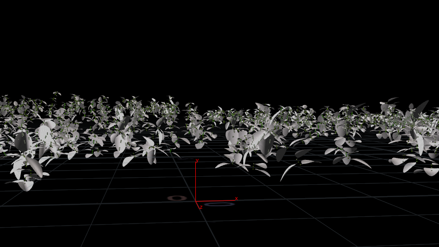
The original version of the sprouts generator was just creating boring old static geometry for the background. It was a similar approach to the hero plant: Leaf geometry randomly instanced onto a handful of L-systems variants, cached to disk and randomly scattered just like the moss variants were. The results were good enough for blurred-out background objects:
Randomized variants of the sprout L-system.
However, once I started doing animated tests, it was pretty obvious that they were static, and with all the commotion happening on the hero plant’s leaves, there needed to be similar movement on the background. The problem was that if I wanted to still use a typical proxy setup here, I would have had to bake out a number of random sprout variants as before, but this time as sequences instead of just single .bgeo files… and then I’d have to randomly offset the timing of each instance so that all of the type02’s or type03’s wouldn’t be animating in sync with each other. With this many different variants, not only would it be an enormous pain in the ass to set up, but all of the memory savings I’d normally get from proxying out these objects would go out the window.
A better approach was to generate all of the L-systems geometry up front, and only proxy the leaves. Inside the sprouts_NEW container, you’ll see a little for-each loop with an Lsystem SOP inside it. The network looks like this:
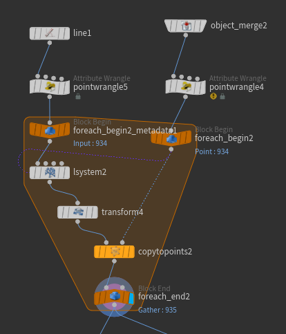
The for-each network that defines each individual sprout.
On the left, a simple line is used as the Leaf J geometry for the L-system. This is to help visualize how the leaves will be oriented before the actual leaf geometry is copied onto those points. On the right, the input points where the L-systems will be scattered get random values for @gens and i@seed. These values are used for the number of generations and the random seed of each L-system copy, via point expressions referencing spare parameters (hence the -1 in the point expression and the little purple line connecting foreach_begin2 to lsystem2). If you haven’t messed with spare parameters yet, check out my earlier blog post on copying and instancing in Houdini.
The rules for this L-system are hideous, as they typically are, but the actual logic behind them isn’t too bad:
Premise: ^(20)FFX(c) B[\(137.5)B][\(137.5*2)B]
Rule 1: X(h):(h>3) = “&(20)\(137.5)~(d)TFX(h-1)
Rule 2: X(h):(h<4) & (h>0) = [\(137.5*h)FB]FX(h-1)
Rule 3: X(h):(h=0) = ~(d)FX(c)
Rule 4: B = J(0.1,0,g,0,0);
The premise is more or less saying “lean over slightly, grow upwards a bit, start growing an X with a counter value equal to variable C (set to 6 in the Values tab), and always end with three B’s at opposing angles to each other.”
Rule 1 is saying that as long as the counter is greater than three, pitch up 20 degrees, twist slightly, wiggle a random amount up to variable D, apply gravity, then grow forward and grow another X with 1 subtracted from the counter.
Rule 2 is what happens when the counter is less than 4. A leaf is branched off after twisting again, then the main stem continues to grow as before.
Rule 3 is what happens when the counter reaches zero: the stem wiggles randomly, then a new X grows with the counter reset.
Rule 4 is just the definition for B: make a copy of Leaf Input J (the first input to the SOP here) and scale it to 0.1.
After the copy, we use the line that defines each leaf to create a normal vector, by subtracting one point from the other per-primitive. We don’t need the other point anymore (the “tip” of each leaf), so we delete it, and then create @pscale and p@orient attributes for the leaves, with the scale defined by a ramp driven by the position of the leaf along the stem. The next Copy to Points operation is a sort of test, to verify that all of the leaves are looking good:
Testing the leaf scales and orientations.
Now to make them move. The first step is to generate the “impacts.” This is when each leaf would be hit by a raindrop. After tossing the packed primitives, an attribute called @impact is randomly generated based on the point number, the current time, and a random seed. The amount of the impact is a random value between 0.5 and 1.0:
float threshold = ch("threshold");
int seed = chi("seed");

if(rand(@ptnum * seed * @Time) < threshold) {
    @impact = fit01(rand(@ptnum * seed * @Time + 9999), 0.5, 1.0);
} else {
    @impact = 0;
}
The threshold value is very low, about 0.003, and is keyframed down to 0.0 before the end of the animation to allow for easier looping. Visualizing @impact gets us this animation:
The “impacts” attribute visualized in red.
Now for some CHOPs! The leaves need to wobble back and forth once they’re impacted, and an easy way to convert these instantaneous impacts to sinusoidal motion is with the Trigger CHOP. Inside CHOPs, if we just plot out the @impact attributes of the first ten points using a Geometry CHOP, we get a graph that looks like this:
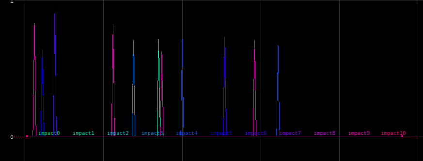
The impact channels for the first ten leaf points, over the animation time range.
The Trigger CHOP uses the MIDI-style Attack, Sustain, Decay, Release pattern to generate a new signal anytime the Trigger Threshold is met. To simulate a raindrop impacting a leaf, the Attack is basically instantaneous as is the Sustain, but with a long release that eases out. A leaf getting hit by a raindrop immediately moves, but the springy motion decays very quickly at first. Applying this Trigger changes the previous impact channels to look like this:
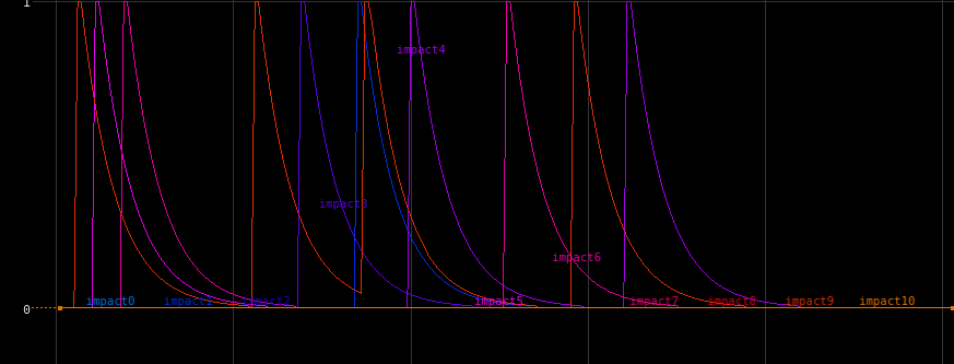
The same channels, with a Trigger CHOP applied.
Now we need to make these channels sinusoidal, so the leaves will bounce up and down. Since these new trigger channels are in a nice 0-1 range, the easiest way to utilize them is to generate a sine wave, then multiply that against these channels, using them as a sort of mask. We’ll use a Channel Wrangle here to generate the wave. Channel Wrangles have slightly weird syntax (no @ at all, and some very different globals to deal with) but they’re very powerful and can potentially multithread. Here’s the code to generate a simple sine wave:
V = sin(T * ch("freq"));
In Channel Wrangle syntax, V is the value of the channel (you always have to write to this global), and T is the current time of the sample. Setting the “freq” channel to 18 and using a Math CHOP to multiply these waves against our original mask channels nets us this graph:
Multiplying sine waves by the earlier impact channels.
This isn’t quite right, though… see how all the peaks and valleys of each channel are aligned? This means that even if impacts are happening at different times, the oscillations are all happening at the exact same time, which will make the leaves look like they’re synchronized. To offset this, we can add a little bit to our Channel Wrangle:
V = sin((T+rand(C)) * ch("freq"));
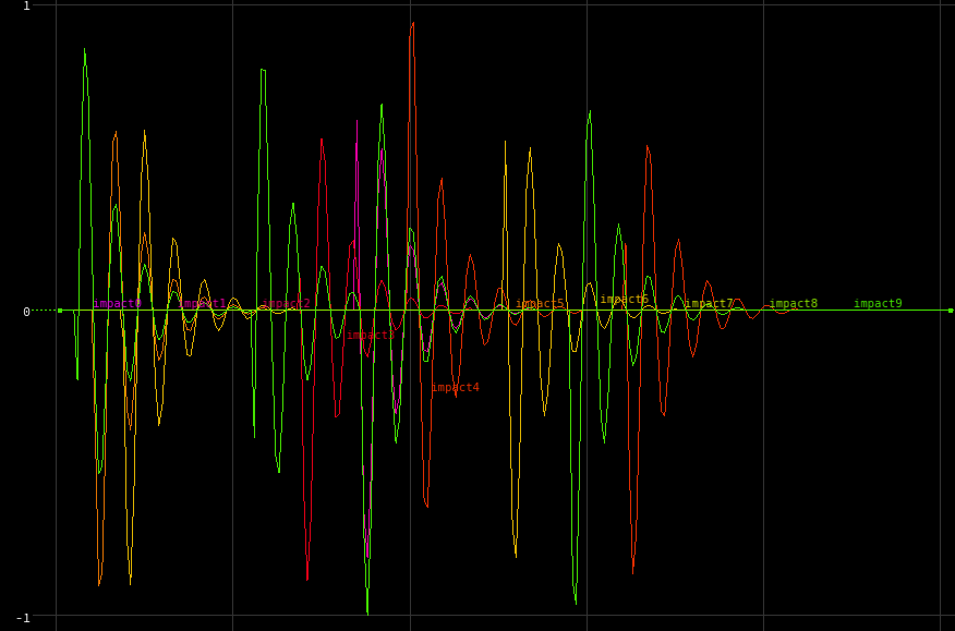
The global C here is the current channel’s index, so each impact channel (each leaf) will evaluate this sine function slightly differently. The result looks like this:
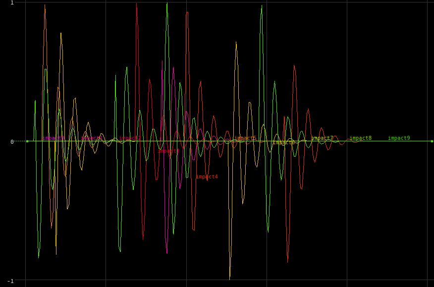
The waveforms after offsetting the sine function.
It’s subtle, but having the more randomized motion is way more believable in the final product. Now we just have to translate these waves into rotations for the leaves. Back in SOPs, the impacts_to_rotations Point Wrangle takes the original copied leaf geometry (as packed primitives) as the first input, and a Channel SOP pointing to our newly-made waveform channels as the second input. The code looks like this:
// make orient quaternion to add to existing rotation
float scaleR = ch("effect_scale");
float impact = point(1, "impact", @ptnum);
vector R = set(impact * scaleR, 0, 0);
vector4 rot = eulertoquaternion(R,0);

matrix3 xform = primintrinsic(0, "transform", @ptnum);
vector4 old_orient = quaternion(xform);

// store orient quaternion for instancing later on
p@orient = qmultiply(old_orient, rot);
matrix3 new_xform = qconvert( p@orient );
scale(new_xform, @pscale);
setprimintrinsic(0, "transform", @ptnum, new_xform, "set");
There’s two things happening here. One part is creating a transform matrix and applying it to the packed primitives, in order to quickly verify that our bounces look good. The other is creating a p@orient quaternion for use in aligning Redshift instances for rendering. It’s only necessary to do both here because Redshift currently doesn’t understand packed primitives as instances; it will render them just fine, but you won’t get the same memory savings that you would from actual instances.
For each packed primitive, we get the matching point from the CHOPnet and get its @impact value. This is converted first into a vector, where impact * scaleR = the amount to rotate in X (in radians), and then that vector is converted into a quaternion via the eulertoquaternion() function. We’ll use this quaternion in a minute.
Packed primitives store their local rotations in a primitive intrinsic called “transform.” If you haven’t dealt with intrinsics before, they’re hidden attributes that aren’t really meant to be modified, but in certain cases they can be modified to great effect. You can look at intrinsics on packed primitives, volumes, and certain other objects in SOPs by going to the Geometry Spreadsheet and clicking the “intrinsics” dropdown in Primitives mode. This matrix is then converted into a quaternion, so we can modify it with the rot quaternion we just made to define the impacts animation.
Combining two rotations with quaternions is easy: just multiply them together. We get the new orientation of each leaf by running qmultiply(old_orient, rot), and bind that to p@orient for use in fast point instancing. This is enough for rendering, but in order to see this right here in the viewport without jumping up to object level, we need to modify this same transform intrinsic. A new rotation matrix is generated from the orient quaternion using qconvert(), then scaled down by @pscale to maintain the scale we already had, before finally applying this value to the original intrinsic using setprimintrinsic(). The result is that the packed primitives are rotating in real-time in the viewport:
The rotations applied to the sprout leaves.
The mushrooms
The mushrooms growing on the stump were a pretty small detail, but there’s a couple of interesting tricks in here worth sharing. The caps themselves are pretty straightforward point-pushing and extrusion. The prims at the bottom of the cap where it is to join the stipe are blasted out, and the edges grouped as “open” for use later. The UVs are also promoted into a duplicate point attribute called v@puv, for use later when distorting the caps.
The mushrooms were only to grow on the side of the stump facing away from the sun, so there’s a Point Wrangle in play to procedurally build a mask attribute. The code is pretty straightforward:
vector dir = point(1,"P",0);
float dot = dot(dir, @N);
@mask = chramp("dot_ramp", clamp(dot, 0, 1));

@mask *= anoise((@P+chv("offset")) * chv("noise_freq"));
The first point that defines dir is just a single sphere primitive, used as a sort of control for determining what side of the stump the shade is on. Computing the dot product of the stump’s normals and the vector between each point and the sphere primitive, then clamping it to a 0-1 range gets us a way to control a ramp parameter to use as a mask. This is multiplied against a simple noise pattern to prevent the growth points from looking too uniformly distributed. Some points are then scattered onto the stump using this mask parameter as the density value, and these will be the growth points for the mushrooms.
The next part is a SOP Solver, which literally grows these points upwards. A Point Wrangle is used to apply some upwards and outwards force to each point, along with some curl noise for randomness. This force is then added to @P for each timestep:
vector curl = curlnoise(@P * chv("curl_freq"));
vector up = {0,1,0};
vector grow = (curl * ch("curl_amt")) + (up * ch("up_amt") + (@N * ch("push_amt") * {1,0,1}));
float bias = fit(@Frame, 1001, 1017, 0.2, 1);
vector force = lerp(@N * ch("push_amt") * {1,0,1}, grow, bias);
v@N = normalize(force);
@P += force;
Trailing this particle system leads to this neat growth animation:
Trailing the mushroom growth solver.
We don’t actually want these mushrooms to animate, so TimeShift-ing the solver to about 17 frames in leads to believable mushroom stipes. These are then given UVs and run through a Sweep SOP, in a similar method to the hero plant from Part 2. A similar “open” edge group is made for the top of each stipe, where they are to be fused with the caps. After merging, these groups are fused together.
Next up, another mask attribute is created by leveraging the v@puv attribute we created earlier. This mask isolates the caps and the top parts of the stipes, so we don’t disconnect the base of any stipe from the stump. The distort_shrooms Point VOP is just adding Turbulent Noise to the point positions of the mushrooms, using this mask attribute as a bias. To make each mushroom a little different, the i@copynum point attribute, generated from the Copy SOP that copied each mushroom, is added to the lookup position of the noise function.
The dewdrops
Nothing super fancy here; the dewdrops are more or less just spheres instanced onto random objects in the scene. In render tests they tended to look a bit static, though, like they were glass beads instead of liquid water, especially when they were out of focus with such a strong bokeh effect. Adding a very slight noise distortion on the top-half of each instanced dew sphere helped make them look more alive.
A close-up of the wobble effect applied to the instanced dewdrops.
To speed up the cook time of the noise for so many spheres, a compiled for-each block was used here. Each individual drop was given a slightly different offset and time offset for the noise function, by creating offset and noisetime attributes on the template points the spheres were copied to. These values were added to the lookup time and position of the noise function that distorts the spheres, per-copy, in a similar fashion to the mushroom noise distortion.
The foreground rain
The foreground rain was handled almost exactly the same as the rain hitting the hero plant; a particle simulation run through a Trail SOP and then meshed into a VDB surface. The only real trick was getting this simulation to loop imperceptibly. The emission rate of the particle sim was again handled through CHOPs… a random noise function was generated to make the rainfall rate just a little unsteady, and then multiplied against a keyframed channel to taper off the rainfall completely by the end of the sequence. This simulation was cached out, then read back in and merged with a duplicate of this same cache, offset by exactly 120 frames (half of the sequence length). The original cache was also run through a Time Warp with Pre- and Post-Extend set to Cycle. The result was rain that more or less looped seamlessly at the 10-second mark.
In order to save render time, the foreground rain was rendered as a completely separate pass from the other elements. All of the other objects were rendered at this point, so the sequence was turned into a self-illuminated plate parented to the camera and refracted through the rain material.
That’s about it! There are probably other little things I’ve glossed over or left out entirely from this breakdown, but feel free to leave a comment here if there are missing parts that warrant an explanation. The rest I hope is decipherable from looking at the HIP file, linked in Part 1. Thanks for reading all of this!