An Even Longer-Winded Guide to Instancing in Houdini

This article is way too long, so here’s the Table of Contents:

1. Introduction
2. Boring Math Background
3. The Copy SOP: Varying Transforms
4. The Copy SOP: Shape Variants
5. Varying Animated Sequences
6. Old School Instancing
7. For/Each Loops
8. Varying Materials
9. Solaris (TBD)
10. Wrap-up (and HIP file, and cats)

Introduction

Ugh, this instancing thing again. The old article is a bit outdated now, and it doesn’t touch on some important stuff about varying instances, especially material properties, so I’m writing an update. I wrote the last guide before I ever released MOPs and I’ve learned a few things about the math since then, and this way I can also tell you to just get MOPs as a way of solving a good chunk of the problems related to copying and transforming things, because I’m a self-serving goblin.

When people start working with Houdini, one of the first things that usually confuses them (assuming they didn’t decide to melt their eyeballs by going straight into simulations) is the myriad different ways that Houdini allows you to make copies of things, and vary those copies. Houdini is a big powerful program that can solve complex problems in many different ways, and it also assumes that you know your way around a lot of basic 3D concepts that most artists aren’t taught at all outside of a bit of high school math that you almost certainly forgot the second you graduated. When you first try to understand how Houdini is trying to ask for input, it’s going to feel like drinking from the fire hose no matter what. Hopefully this guide will make that fire hose just a little less… hose-y.

Anyways, this guide is going to try to answer these important questions:

• How do I randomly (or not randomly) transform copies of things?
• What even is a transform and why do I care?
• How do I vary what object is copied to each point?
• How do I vary specific properties of each object?
• How do I change properties of shaders per-object?
• Is there an easier way to do any of this? (sometimes)

We’ll unfortunately have to start with a little bit of background to understand the weapon that is the Copy SOP.

Boring Math Background

A lot of what the Copy to Points SOP and other forms of instancing in Houdini are about is varying transforms of things. So WTF is a transform? A transform, or transform matrix, is a neat little box of numbers that defines something’s position, orientation and scale in space. Transforms are used literally everywhere in computer graphics, so it’s important to at least understand the basics. In Houdini, there’s two kinds of transform matrices that you’ll see most often: a 3×3 matrix, or matrix3 in VEX, and a 4×4 matrix, also just called a matrix in VEX. With Copy to Points, you can potentially use both these data types to define where copies go, but in practice most of the time you’re going to be dealing with 3×3 matrices.

A 3×3 matrix describes the orientation and scale of an object in space. What about position? In Houdini, we often use the @P vector attribute to handle the position of a point instead. This is often easier to work with and to read than a 4×4 matrix, which includes position.

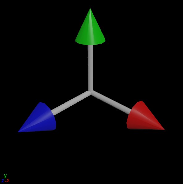
Okay now what’s a matrix? It’s literally just a stack of vectors. In the case of a 3×3 matrix, what you have is a cute little stack of three vectors, each vector telling you what an object’s “forward” (+Z) direction is, what the “up” (+Y) direction is, and what the “side” (+X) direction is. The length of the vectors describes the scale of the object along each of those axes. You can think of it like the familiar gnomon you see in most 3D programs, but instead of showing you the orientation of the world, it’s showing you the local orientation of the object.

An important matrix you might see frequently is the identity matrix, which is basically a “do-nothing” matrix. Here’s what it looks like:

[1, 0, 0]
[0, 1, 0]
[0, 0, 1]

What this means literally, reading left to right, top to bottom, is:

• X is X.
• Y is Y.
• Z is Z.

This means that the matrix is exactly the same as the world matrix (or whatever the matrix’s parent is), so there’s effectively no transformation happening. Now imagine you see a matrix like this:

[1, 0, 0]
[0, 0, 1]
[0, -1, 0]

This matrix is saying that X is still facing towards world X, but Y is now facing towards Z, and Z is facing towards -Y. This sounds insane when described in this way, but really all we’re seeing is a 90 degree rotation around the X axis.

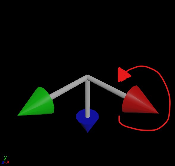
Most of the time you’re not going to get pretty numbers like (0,0,1), but this is conceptually how you’re defining the orientation of any given copy in space. The first vector says “this points to my side”, the second says “this points up”, and the third says “this points forward”. Houdini (or whatever your application is) does the rest.

An important note to take from all of this is that when you’re preparing geometry to be copied to anything, you will want it to be aligned to the world such that the forward axis of your object is facing +Z, and the up axis of your object is facing +Y. What exactly forward and up means for your object is subjective, but you will need to be aware of that decision before copying.

A very cool thing about matrices, and one of the reasons they’re used everywhere in 3D, is that you can multiply vectors by matrices to transform them. For example, if you multiply the vector (0,0,1) by the matrix above that represents a 90 degree rotation around X, you’ll end up getting the vector (0, -1, 0). You can also multiply matrices by each other! This is how most of 3D works… a series of multiplications, transforming points and normal vectors into their final positions and directions in space. A parent/child relationship in a transform hierarchy is just a series of matrix multiplications applied in order.

The order in which you multiply matrices determines the “space” you’re working in. If you have a matrix A that describes a random orientation and you have another matrix B that describes a 90 degree rotation in X, if you multiply A * B you will get a 90 degree rotation around X in world space:

Conversely, if we switch the order of multiplication and do B * A, we get a 90 degree rotation in the local space of our initial orientation:

If you want to transform one object’s matrix into the local space of another, it’s just outMatrix = matrixA * invert(matrixB). Cameras have their own special projection matrices that transform polygons into viewport space for rendering. It’s matrices all the way down.

Forward and Up

A lot of Houdini scrubs (I say this lovingly) will do a simple particle animation and wonder why things look weird or jittery when they copy things to their particles or animated meshes. Objects will flip or jitter, or will be rotated in strange ways even though Copy to Points is using the velocity of each particle (or point normals) to orient each copy. The reason for this is that, as demonstrated above with our friend the gnomon, orientation is described by three vectors, not one. So what exactly is happening here?

Houdini, in a somewhat misguided effort to be friendly and helpful to you, is making an educated guess as to what your “up” vector might be. If all it has is a forward vector to work with, how is it supposed to know how the copy should be twisted around that vector? It has no clue, so it guesses based on a fancy math concept called a dihedral. Basically, it computes the difference between the “forward” axis you gave it (N or v, usually) and applies that same difference to world up (+Y) and just rolls with it. Other applications like Maya or Blender will explicitly demand an up vector when trying to orient things, such as with an aim constraint, but Houdini blissfully just bullshits something if you don’t give it better instructions.

If you do provide an up vector, the simulation is much more stable (but not perfect):

If you’ve been paying attention, you might be wondering “well what about that third vector that makes up a matrix?” Why do we only need two vectors to define the orientation and not three? The reason for this is that for a transform matrix to be (for most purposes) valid in 3D, it needs to be orthonormal, meaning each axis that makes up the matrix is more or less perpendicular to the other two axes. If you have a forward and an up vector that are, for the most part, facing in perpendicular directions, you can use a fancy operation called the cross product to automatically compute that third vector. The cross product creates a new vector that is orthogonal to the first two vectors, and the three of these vectors together creates a matrix.

So why the flipping, especially when objects are traveling straight up or down, even with that up vector? This is happening because the forward vector (remember, this is the direction of motion!) and the up vector are too similar to each other. It becomes harder and harder to compute a vector that’s orthogonal to the other two as the first two vectors get closer and closer, and finally that third vector will flip to the opposite side as the two vectors cross each other. Because our up vector is a constant (0,1,0), if the velocity of any given particle becomes too close to (0,1,0) or (0,-1,0), some instability will result when computing the orientation.

Quaternions

One other way you’ll see orientations defined in Houdini (and elsewhere in 3D) is as quaternions. My most important piece of advice regarding quaternions: don’t bother trying to understand the numbers. Quaternions are truly wizard shit and no normal human can understand the values intuitively. That said, they happen to be a very clever way of encoding an orientation as a 4-dimensional vector (as opposed to your usual 3-dimensional vector) and they also have the unique property of being very easy to blend together. This makes them great for smoothly rotating from one direction to another over time, and because of this property they’re used all over the place in game engines and elsewhere when aiming and orienting things.

Quaternions can easily be generated in VEX via an “angle/axis” constructor. You define an axis of rotation and an angle in radians and get a quaternion:

// create a 90 degree rotation around world Y
vector4 rotation = quaternion({0,1,0}, radians(90));

You can then use this quaternion to rotate vectors, or accumulate multiple rotations by multiplying quaternions together:

 // create a 90 degree rotation around world Y
vector4 rotation = quaternion({0,1,0}, radians(90)); 
// rotate the N vector with a quaternion
@N = qrotate(rotation, @N);
// "add" this rotation to the existing orientation in local space
p@orient = qmultiply(p@orient, rotation);
// reverse the terms and you "add" the rotation in world space
p@orient = qmultiply(rotation, p@orient);

In Houdini, and many other 3D applications, quaternions can be easily blended between via the slerp function, short for “spherical linear interpolation”. If you have two orientations, A and B, and want to blend to halfway between, you could just say slerp(p@A, p@B, 0.5); and you’ll get an orientation exactly halfway in between. It’s really amazing stuff. Additionally, specifically in Houdini, you can slerp 3×3 matrices! This can be really handy for blending packed transforms and KineFX joint values, as long as you don’t mind a little VEX.

If we wanted to avoid the flipping present in the above examples entirely, a good way to do it would be to use POP nodes to smoothly blend the orientation towards the direction of motion, taking into account the entire orientation of the object on each timestep relative to the previous timestep (instead of just forcing an arbitrary up vector on each individual frame with no continuity between frames, which is how SOPs works). A POP Lookat DOP with the target set to v@v will set the orient quaternion attribute on your particles and interpolate them nice and smooth over time:

It’s important to note that the use of quaternions isn’t the only thing preventing this simulation from flipping or otherwise acting erratically; it’s also the fact that the simulation is able to look at the orientation of the previous frame and make small adjustments over time, rather than computing each frame’s orientation “just-in-time” independently of the previous frames. This potential discontinuity between frames can’t be avoided without the use of some kind of solver or event loop (such as the loop you’d inherently get in a game engine).

Quaternions and 3×3 matrices are pretty similar to each other, and in VEX you can convert between them using the qconvert and quaternion functions. The important difference is that quaternions can’t encode scale, and in the end your copies will be using transform matrices under the hood to determine their position, orientation and scale. They’re just a great tool for handling smooth blending between rotations.

The Copy SOP: Varying Transforms

Okay, with all that boring stuff out of the way we can actually talk about Houdini. When you’re copying objects to points using the Copy to Points SOP, the way you determine the transform of each copy is by using what Houdini calls template point attributes. These point attributes control the position, orientation, and scale of each copy. There are a lot of these attributes that you can use, defined in this help article. The most important ones are:

• v@P, the position of each point
• v@N, the “normal” or “forward” vector
• v@up, the “up” vector
• f@pscale, the uniform scale
• v@scale, the scale for each individual axis
• p@orient, a quaternion that defines the full orientation

Copy to Points will read these attributes in a specific order of priority to determine the transform of each copy generated. The help article goes into detail on the order of operations.

Polygons and Packed Primitives

When you copy objects to points, by default you just get copies of your original object, likely expressed as polygon geometry. Copy to Points uses the template point attributes of each input point to determine the overall transform of each copy, but that transform doesn’t really “exist” after the fact; it’s baked into the results. For example, here’s a default pig head copied onto a grid. Check out the Info window:

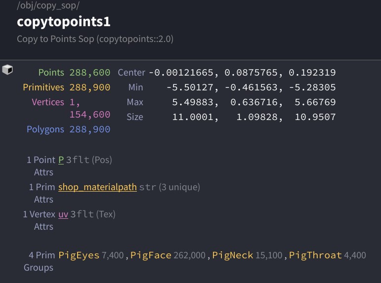
The first thing to notice is that there’s a lot of polygons. Even though these pig heads are all functionally identical to each other, they are just a mess of points and polygons as far as Houdini is concerned… without other attributes or groups in play, there’s no way to differentiate between them. Additionally, even if we used template point attributes to randomize the orientation or scale of each pig head, that information is lost after the copy operation.

Now enable “Pack and Instance” on the Copy to Points SOP. Check the info window again:

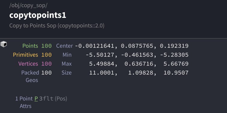
In this case, we’ve told the Copy SOP to encode each of these objects as a packed primitive, which is a kind of instance in Houdini. This is great for several reasons: first, this means that Houdini doesn’t have to work nearly as hard when displaying or rendering this geometry, because it only has to remember what one pig head looks like rather than one hundred of them; second, this means that you can individually manipulate these pig heads downstream of the Copy operation as “objects” rather than as “big messes of point data”.

Primitive Intrinsics

If you play around with these packed objects, maybe with an Edit SOP, you’ll notice that you can pretty easily move them around, rotate them, scale them, whatever. But where is the information about each head’s transformation stored? It’s encoded as primitive intrinsic attributes, hidden away in a special part of the Geometry Spreadsheet. To the Spreadsheet:

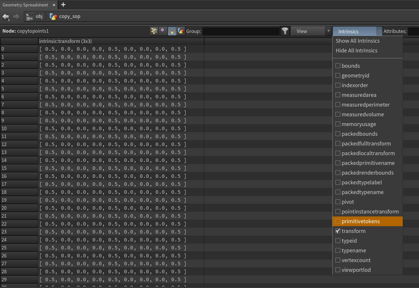
If you open up the “Intrinsics” dropdown (this is only visible in Primitives mode), you’ll see a whole list of secret attributes that define all kinds of interesting things about each object. For packed primitives, the most important one is the transform intrinsic, a 3×3 matrix that probably sounds familiar by now. In the screenshot above, note that the matrix looks just like the identity matrix demonstrated earlier, except that 0.5 is seen in place of 1.0… this is simply because the pscale of the template points before the copy operation was set to 0.5, scaling the pig heads down by 50%. It’s literally just multiplying those vectors!

Some of these intrinsics can actually be modified manually, but it must be done in VEX and can sometimes be a bit tricky. You can check out the setprimintrinsic function if you like and try to have a play with it. MOPs messes with primitive intrinsics extensively to transform packed primitives after they’re already created (in addition to transforming template point attributes).

The only downside to packed primitives, generally speaking, is that they’re immutable. You can’t modify the geometry inside, or peek at their packed attributes, even though they still exist in there. If for whatever reason you need to deform one of those pig heads, you’re out of luck unless you use the Unpack SOP to unpack the geometry, losing out on the instancing performance.

Tweaking template point attributes

Everything up to this point is great in theory, but how do we actually set these attributes? This is where things can start to get a little tricky, and there’s a lot of different ways to do this depending on how busy and/or technically inclined you are. I’ll show a few of the basic ways to manipulate these attributes in (mostly) human-readable ways. First, here’s our initial conditions: a simple grid of pig heads as packed primitives. The grid is facing +Y, and so I’ve manually set the N attribute on the grid points to face +Z with the expression v@N = {0,0,1};. Here’s what it looks like from above:

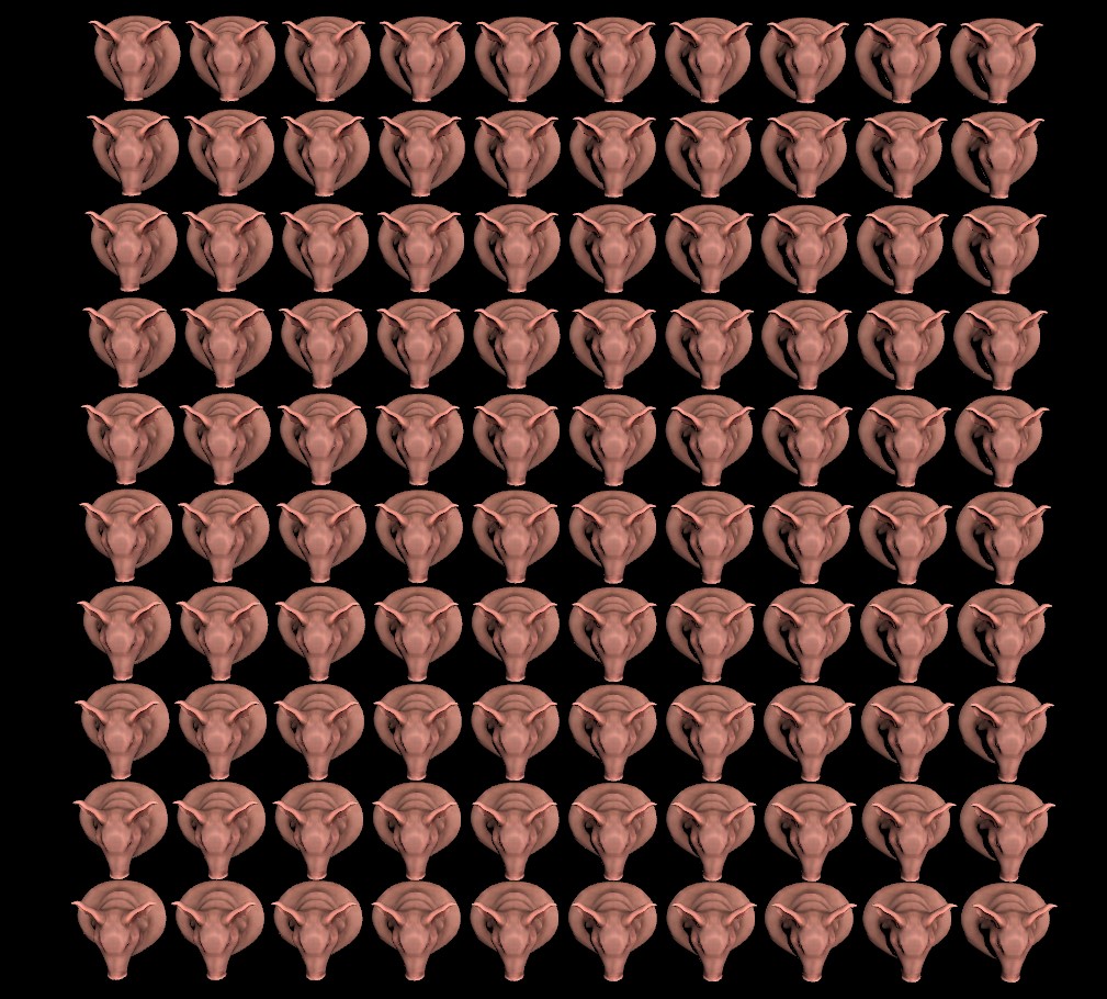
Adjusting the uniform scale of these guys is pretty straightforward with the Attribute Adjust Float SOP. With pscale as the Attribute Name, you can just randomly set the pscale value between a minimum and maximum range and get this:

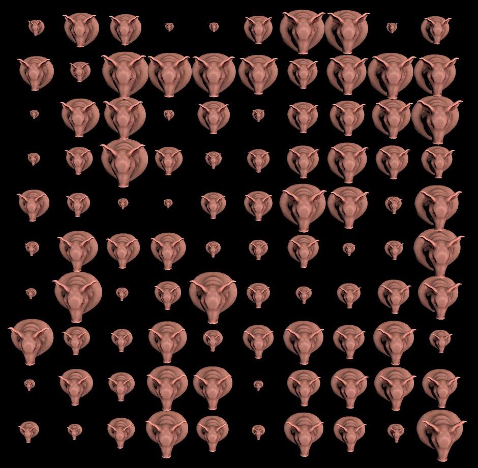
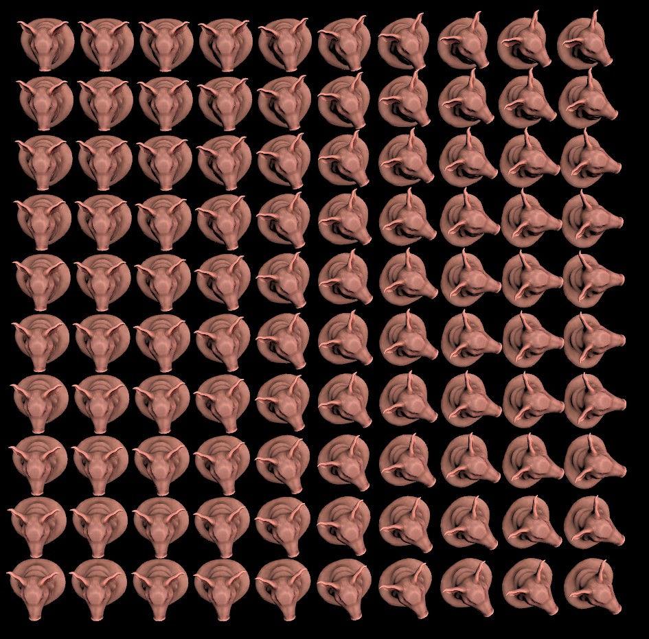
With a slightly more complicated set of parameters, we can use Attribute Adjust Vector to rotate the N attribute randomly around the Y axis. The adjustment is set to “Direction Only” so we don’t accidentally scale N, the operation is set to Rotate, and the axis of rotation is (0,1,0), meaning +Y. This twists the forward axis of each copy around Y:

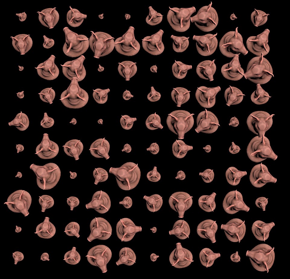
We can just scramble the orientation entirely by using the Attribute Randomize SOP on the orient attribute. Set the Dimensions parameter to 4 (because orient is a quaternion!) and you get something like this:

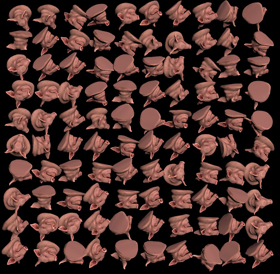
These tools are all great, and if you can believe it, some of them were only recently introduced… Attribute Adjust was only added in 18.5! You can imagine how much of a headache it could be to set N or up with any level of control without these nodes. That said…

• What if you wanted to rotate each object by a slightly different amount?
• What if you wanted to randomize rotation around a specific local axis for each object?
• What if you wanted to aim these objects towards a target?

There are of course ways to do this using existing tools in Houdini, but it can start to get trickier from here. For example, if you wanted to rotate each object around the same axis by a controlled amount, like a wave, you could create an attribute on your points based on the distance to a point with the Mask from Target SOP, and use that to drive the rotation of the N vector. This is where that prerequisite math knowledge starts to come into play. Here’s an example:

matrix3 m = ident(); // create our "empty" starting matrix
vector axis = {0,1,0}; // the axis to rotate around
float angle = radians(90); // a 90 degree rotation
angle *= @mask; // multiply the angle by a "mask" float attribute we created with the Mask from Target SOP
rotate(m, angle, axis); // rotate the matrix around the axis 
v@N *= m; // multiply N by this matrix, this applies the rotation!

This works great, but it does mean that you need to know enough VEX (and enough of the prerequisite math) to set up this rotation matrix, define an axis and angle, turn that into a matrix to modify the existing N attribute, and multiply N by this matrix to transform it. Now imagine a scenario where the pig heads are arranged in a spherical pattern and you have to rotate them around their own local Y-axes, or you want to randomize orientations but mask the values like in the above example. You’re going to start leaning on VEX a lot more often than most people would like.

The short answer, of course is use MOPs. It comes with lots of human-friendly tools to transform things in specific or random ways, in the local space of each object or in world space, blended by all kinds of mask tools ranging from primitive shapes to audio clips. I wrote MOPs and this is my blog so I’m going to toot my own horn as much as I please. (Seriously though, it makes this stuff much easier, even Disney uses it, save yourself the headache.)

The Copy SOP: Shape Variants

Everything up to this point has been about leveraging template point attributes to modify the transforms of copies, meaning the position, orientation and scale. If you want to start varying what object is copied to each point, thankfully Houdini as of version 18.0 has made what used to be an absolute nightmare into a comparatively straightforward process.

Copy to Points has a parameter called “Piece Attribute”, that can correspond to a primitive attribute on the geometry to copy and a matching point attribute on the template points. If some geometry has the name attribute with a value of pighead, and a template point has a matching name attribute with the same value, that named geometry will be copied to that specific point.

In Houdini 18.0 it could sometimes be a little tricky to create the matching attribute on the template points, but in Houdini 18.5 we got the very useful Attribute from Pieces SOP. By feeding this node all of the various named geometry we might want to copy, along with our blank template points, Attribute from Pieces provides a number of random and non-random methods of assigning the matching name attribute to the template points. The network to set this up looks like this:

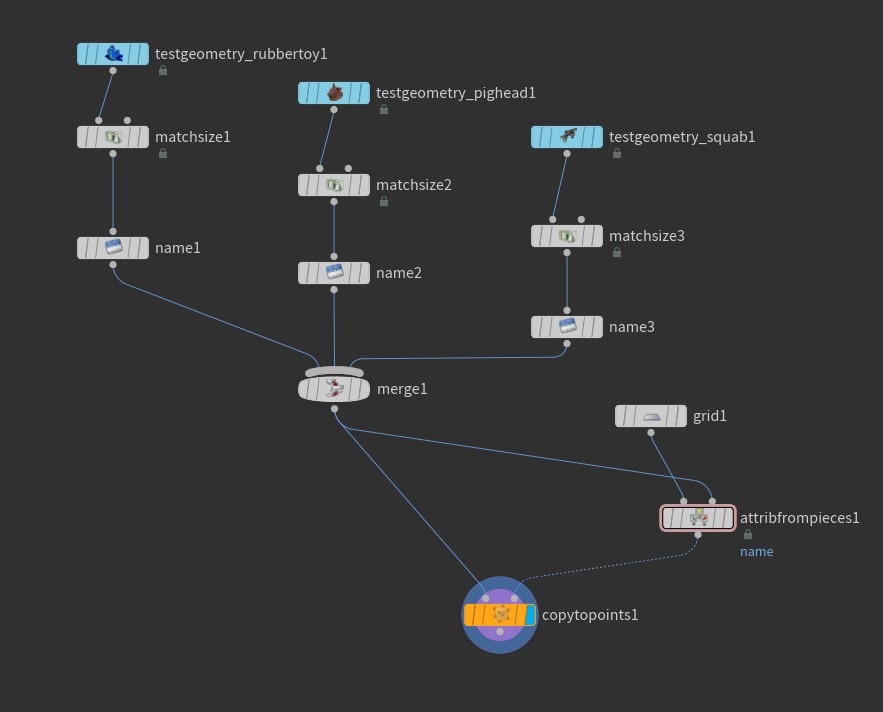
This workflow is very powerful and worth familiarizing yourself with. In prior versions of Houdini you could only do this using copy stamping (which is now fully deprecated and should be avoided) or using complex For/Each Blocks that we’ll go into later for other reasons. MOPs introduced the MOPs Instancer to make this process more human-centric, and it still functions perfectly well, but it’s not quite as necessary anymore thanks to the Copy to Points SOP’s Piece Attribute and Attribute from Pieces SOP.

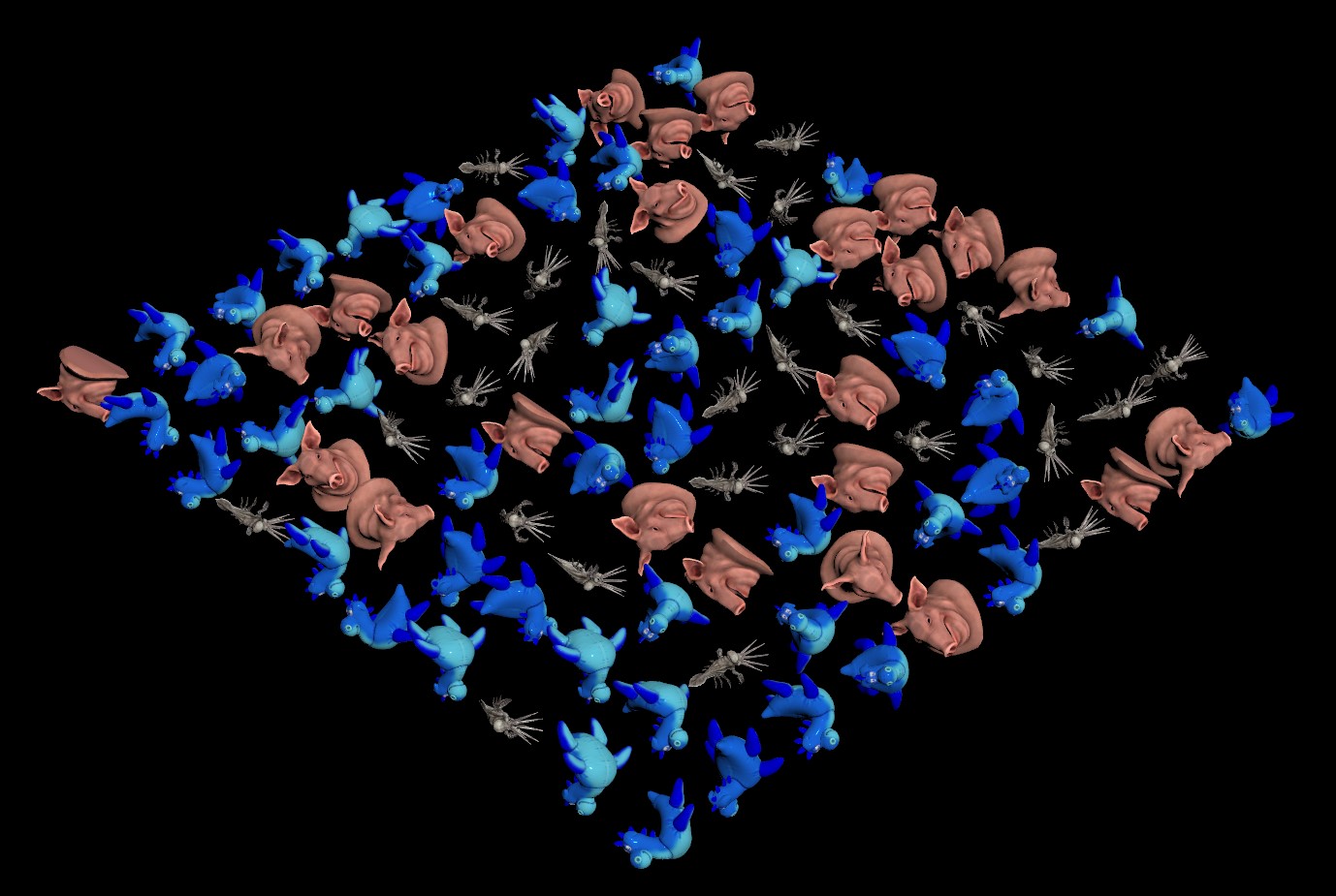
Of course, if you want to do this sort of thing manually, all you need are matching string or integer attributes between your primitives to copy and your template points. There’s endless ways to accomplish this, though most of them will require a tiny bit of VEX here and there. For example:

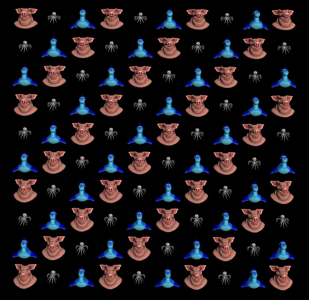
The above configuration is done just using a bit of VEX instead of Attribute from Pieces. A Primitive Wrangle was used in place of each Name SOP from the previous example, setting i@variant to 0, 1 or 2 for each shape. A Point Wrangle is used on the template points with the following code:

// get the relative (0-1) position of each point in the overall bounding box.
vector bbox = relbbox(0, @P);
// fit the X component of these bounds from 0-1 to 0-2.
float x = fit01(bbox.x, 0, 2);
// round to the nearest whole number and cast to an integer.
i@variant = int(rint(x));

You could build similar setups using noise functions, waveform functions, texture maps, volume samples, you name it. MOPs Falloff nodes and the MOPs Index from Attribute SOP are also purpose-built to handle this sort of thing. In the end, all you need are matching numbers, and any number of tools exist to help you create them now.

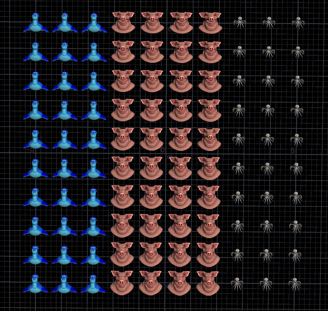
Varying Animated Sequences

Another common type of instance manipulation involves instancing animated sequences; for example, a simple flock of birds, or a bunch of flowers blooming, or a crowd of people going through a simple walk animation (not a crowd of Houdini agents, which is much more complex). While in theory you could handle this with the “piece” or “variant” attribute mentioned above, there’s another way: packed sequences.

There’s two primary types of packed sequences you’ll deal with in Houdini: packed disk sequences and packed Alembics. Packed Alembics are effectively just Alembic files streamed from disk, similar to how render engines like VRay or Arnold have Alembic “procedurals” that can read and process the geometry at render time. They otherwise more or less act like regular packed primitives, except that they have a new secret hidden intrinsic attribute: abcframe. Note that despite the name, abcframe doesn’t actually refer to the current frame of the sequence; it refers to the time of the sequence, in seconds!

Let’s say you have a cached walk cycle, written out as an Alembic. You can copy the packed Alembic to points just like anything else:

Of course, Alembics don’t have any concept of “cycling” when packed like this, so not only are they all walking the same way, but they stop at the end of the sequence. Let’s fix both of those problems.

In this particular walk, the cycle is exactly 25 frames long. We first want to add a random offset to the evaluated time for each packed Alembic, and then we want to loop the evaluated time if it goes past the total length of the sequence:

// create random time offset value
 float offset = rand(@ptnum);
 float out_time = @Time + offset;
 // loop the sequence. this walk is 25 frames long, or 25/24 FPS = 1.0416 seconds.
 float cycle = 25 * @TimeInc;
 // the modulo operator will cause the value to loop back to zero after it passes the cycle length.
 out_time = (out_time % cycle) + @TimeInc;
 // set the abcframe intrinsic.
 setprimintrinsic(0, "abcframe", @ptnum, out_time);

The modulo operator (%) comes up a lot whenever you’re trying to create a looping or cycling behavior. We add a random value, up to a second, to the current evaluated @Time (this is the playbar time, not the time for each sequence). We then figure out the total length of the sequence in seconds by multiplying it by @TimeInc, 1.0 / FPS. Using the modulo operator to loop the offset time value by the length of the sequence creates an endless cycling time value. Then we just use setprimintrinsic to set abcframe to that computed value:

Packed Disk Sequences are very cool and easier to deal with in some ways. Instead of dealing with time values in seconds and setting abcframe, Packed Disk Sequences use frame values to set index. Additionally, you can set index to be fractions of frames, and Houdini will interpolate between frames for you! Houdini also knows to sample surrounding frames when rendering in order to properly apply motion blur. Also very helpfully, Packed Disk Sequences have built-in cycling behaviors to choose from! Sounds perfect, right?

Well, mostly. The biggest downer is that Packed Disk Sequences have very limited support with third-party render engines… as far as I know, only Mantra can properly utilize all of these benefits without having to unpack (and bloat your memory requirements as a result).

The s@instancefile attribute

There’s one more way to handle instancing file sequences, and it’s compatible with most third-party engines, but it’s a bit cumbersome to work with. The instancefile string attribute allows you to directly path to a cache on disk that you want to render. If you’re dealing with a native render engine, you can just specify a path to a .bgeo file on disk. Even better, though, some third-party engines like Redshift allow you to instance their native geometry format via instancefile. This means that you can directly instance .rs proxy files, or sequences of proxy files! The downside is that, for a sequence, you’d have to construct these strings yourself in either Python or VEX, and as you can imagine, this can get pretty annoying:

// get the base path of the sequence, up to the frame extension
string base = "c:/users/henry/desktop/walk";
// get the current frame number we want to load
int num = @Frame;
// concatenate the base path and the frame number (with 4 digits padding), and add the .rs file extension
s@instancefile = sprintf("%g.%04d.rs", base, num);

The sprintf function is one of my favorites in VEX, and it’s doing all the heavy lifting here. In the string to substitute, the %g means “just substitute whatever here, I’ll guess what you want”, and corresponds to the first argument after the string, base. The %04d in the string means “a number is going to go here with four digits of padding”, and corresponds to the second argument after the string, num. It smashes all this together into a string, adds .rs at the end, and now you have your instancefile attribute ready to go. You won’t see anything in the viewport, but Houdini will instance the file to those points at render time.

If you don’t see yourself wanting to type all of this stuff out in production, fear not: there’s a MOPs solution called MOPs Set Sequence Time. Set Sequence Time allows you to simply input an attribute or an offset value, and regardless of what kind of sequence you’re using (Alembic, Packed Disk Sequence, or instancefile path) it will figure out the rest, including cycling behaviors.

Old School Instancing

There’s another very old-school way to instance geometry in Houdini that existed long before packed primitives were introduced. Rather than use the s@instancefile attribute to instance a cached geometry from disk, you can use s@instance to instance OBJ-level containers to points. In general, packed primitives and the Copy to Points SOP are a much more flexible and useful workflow, but there’s one important reason why you might need to use this older method: third-party renderer support. While there are some render engines like VRay and Redshift that support many of the prior instancing methods discussed here, others do not have this kind of support, and you’ll have to deal with OBJ containers until they add it.

To enable this behavior, you either need to create an Instance OBJ, available from the Tab menu, or you need to manually add the required instancing parameters to any Geometry network via the Edit Parameters interface. On the left, look for Render Properties and find the Instancing tab under the Mantra tab, then drag the Instancing tab into the right-hand parameter list. The Instance OBJ is really just a generic Geometry network with these properties added for you, and an Add SOP inside. Either works.

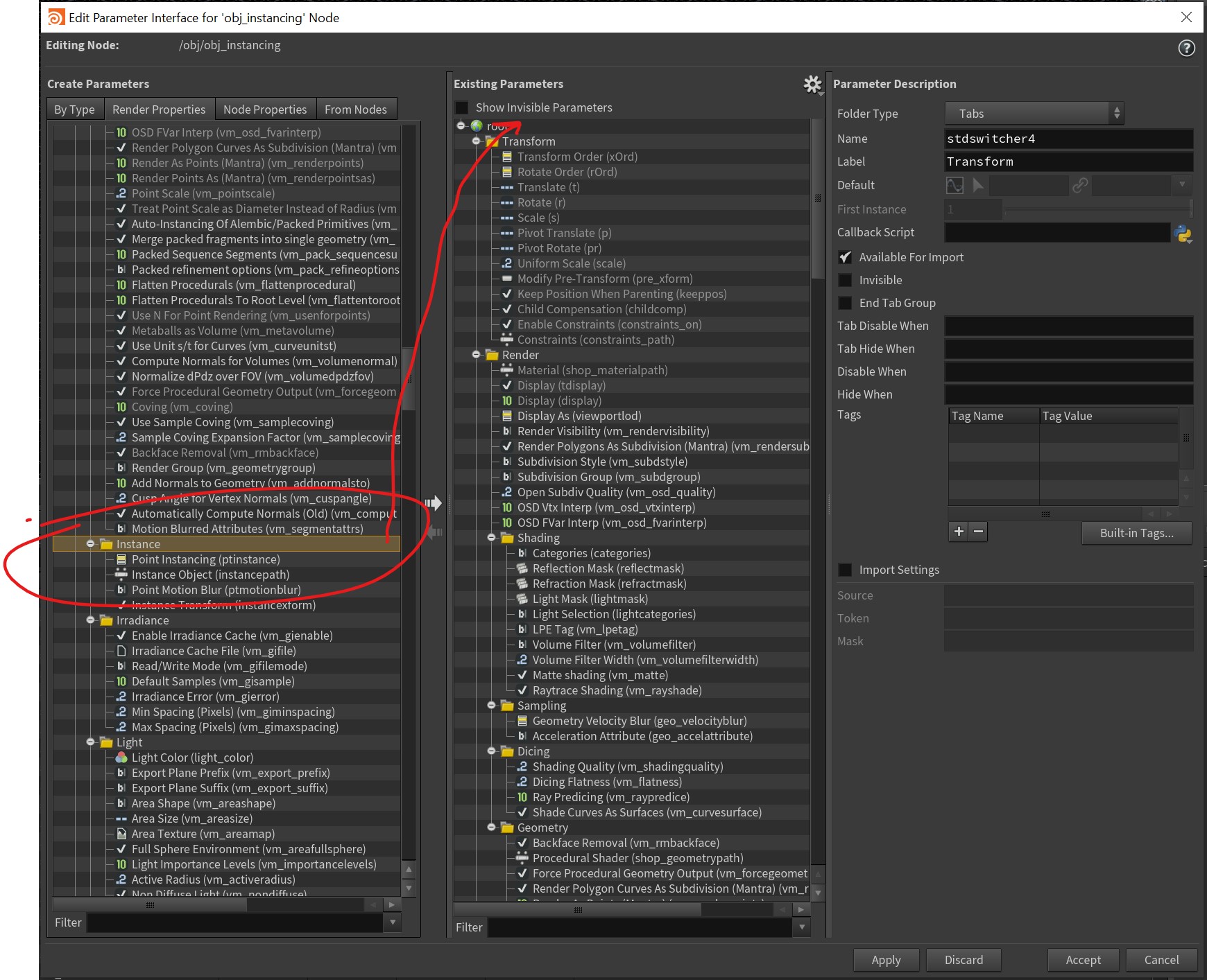
The next step is to open up the newly-added Instance tab in the node properties, and set the Point Instancing parameter to Fast point instancing. This will enable the use of the s@instance attribute on any points inside. You might notice there’s also an Instance Object parameter here. If you were only instancing a single object, you could use this, but in my experience it’s pretty rare you’d be both A.) instancing just one object, and B.) using old-school point instancing. The s@instance attribute should generally be used instead.

Once you’ve set this up, you just need to make sure that each of the objects you want to instance is neatly set up inside its own Geometry container. There’s unfortunately no built-in way to automate this, though if you used the MOPs Instancer, there’s a shelf tool called MOPs to Point Instances that will automatically create these for you.

Once that’s done, the only thing left to do is to create the point attribute values on the points inside your main container. The rules for the template point attributes are otherwise exactly the same as the Copy to Points SOP; @pscale, @N, @up, and so on. You can dynamically generate paths in a similar way as described above with the s@instancefile attribute. Here’s some example VEX:

// generate random integer between 1 and 3
 int rand = int(rint(fit01(rand(@ptnum), 1, 3)));
 // create a path to a random instance container "test_#"
 string path = sprintf("../instance_containers/test_%g", rand);
 // instance paths must be absolute! no relative paths allowed
 s@instance = opfullpath(path);

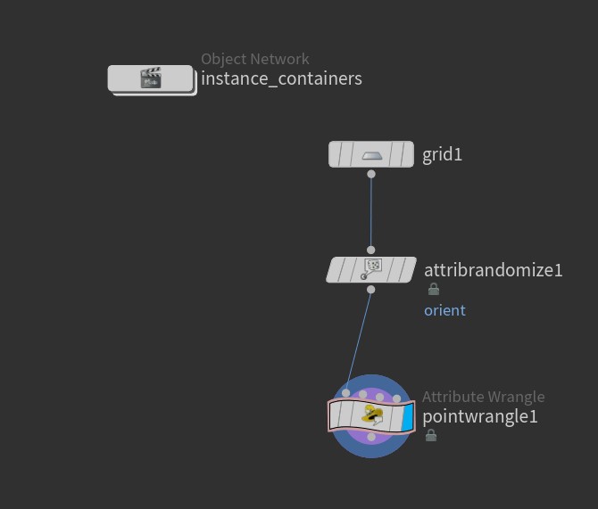
Note that the path is literally just the path to the Geometry container you want to instance, in Houdini terms, and that it must be an absolute path (meaning, starting from /). The opfullpath function is very helpful here! The instance_containers node in this example is an Object Network containing the Geometry networks to instance, named test_1 through test_3.

Note that you won’t actually see anything happening in the viewport. This geometry is created at render time and doesn’t actually exist otherwise. However, if you jump out of the Geometry network you’re in and view at the OBJ level, the viewport will show you a preview of your instances (assuming you set everything up correctly):

For/Each Loops

Here’s where things start to get a little hairy. Let’s say you want to copy a randomly generated object to a bunch of points, like a simple L-system, and you want each copy to be different. You could just animate your random seed value(s) and write the results to an animated sequence, and control the sequence number using the methods described above. This is a totally valid workflow and worth leaning on! But you might be in a situation where there’s too many variations to deal with, or the caching to disk becomes too cumbersome, or some other production reason pops up that makes sequences a problem.

Enter the For/Each Block in Houdini.

In ye olden days, Houdini artists would accomplish this kind of behavior using something called copy stamping, which allowed you to “stamp” arbitrary variables on the Copy SOP to individual copies. These stamp variables could be read upstream in the SOP network, before the copy operation, using the stamp() expression, allowing for each copy to have a different value for the expression. This was very cool, but it’s important to emphasize the was. This is a deprecated workflow and is no longer supported. Don’t do it.

Instead, we can accomplish something similar via For/Each blocks. We loop over each point we want to copy something to, and then we can use the point expression to fetch values that we might want to use to drive parameters in the loop, such as a random seed or an extrusion depth.

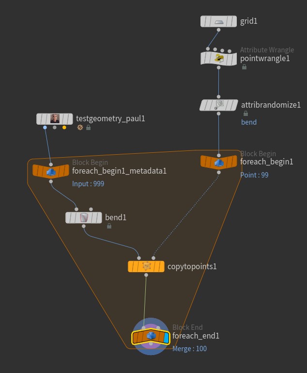
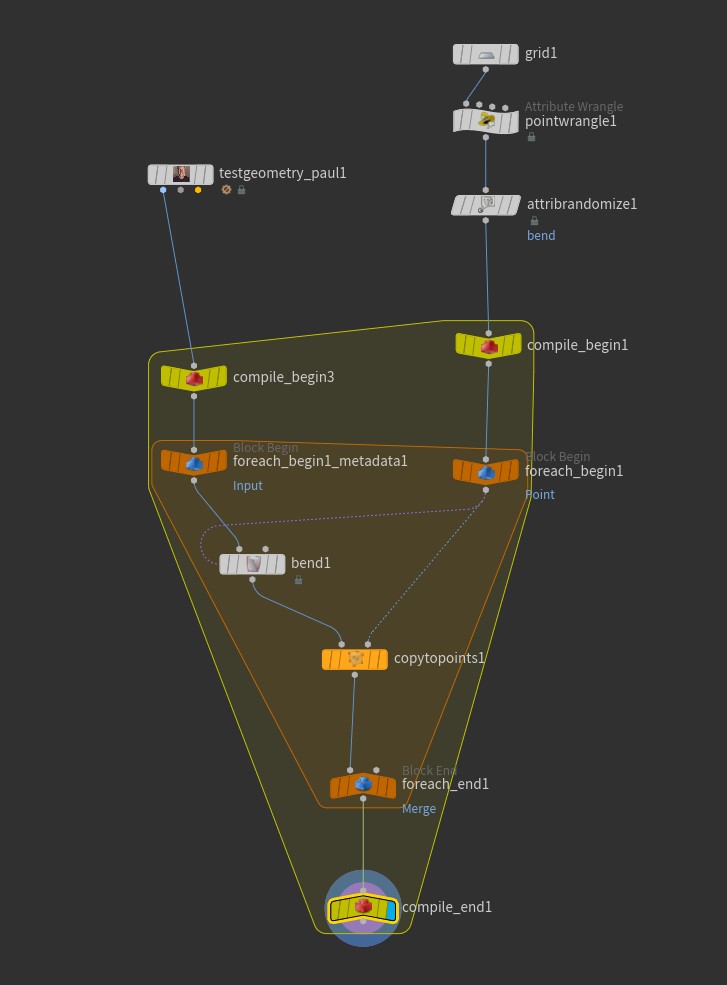
Here’s the start of a simple example. We have a Paul SOP that we’re copying to points on a grid. We want each of these Pauls to run through a Bend SOP, and each copy will be bent by a random amount. The Bend SOP is mostly default; the Capture Direction is set to {0,1,0} but otherwise untouched.

Instead of just copying Paul to all the points as a whole like we normally would, we’re using a For Each Point block to copy over each point, one at a time. If you click on the Block End node after creating a For Each Point block from the Tab menu, you’ll see that the Iteration Method is “By Pieces or Points”, and the Gather Method is “Merge Each Iteration”. This means that we’re considering one input point at a time independently of the others, and after the loop is completed, all of the results are merged together. (For/Each loops can also be used in Feedback Each Iteration mode, which acts like a kind of solver, each loop working over the results of the previous.) The other nodes are just generating a random bendpoint attribute between -90 and 90, currently unused, and setting an initial pscale and N attribute for copying:

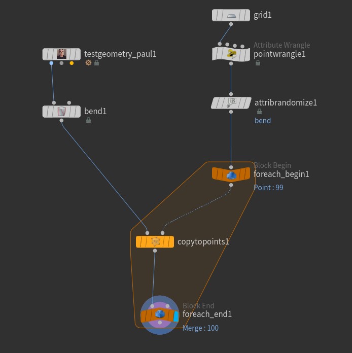
The node that we want to modify per-loop is the bend1 node. Right now it’s not going to evaluate differently in each iteration of the loop. To enable this behavior, we first need to create another Block Begin node. If you select the existing Block Being, there’s a little button called “Create Meta Import Node.” Click that, then select the new node and set the Method parameter to “Fetch Input”. Then wire up the Bend SOP after that node:

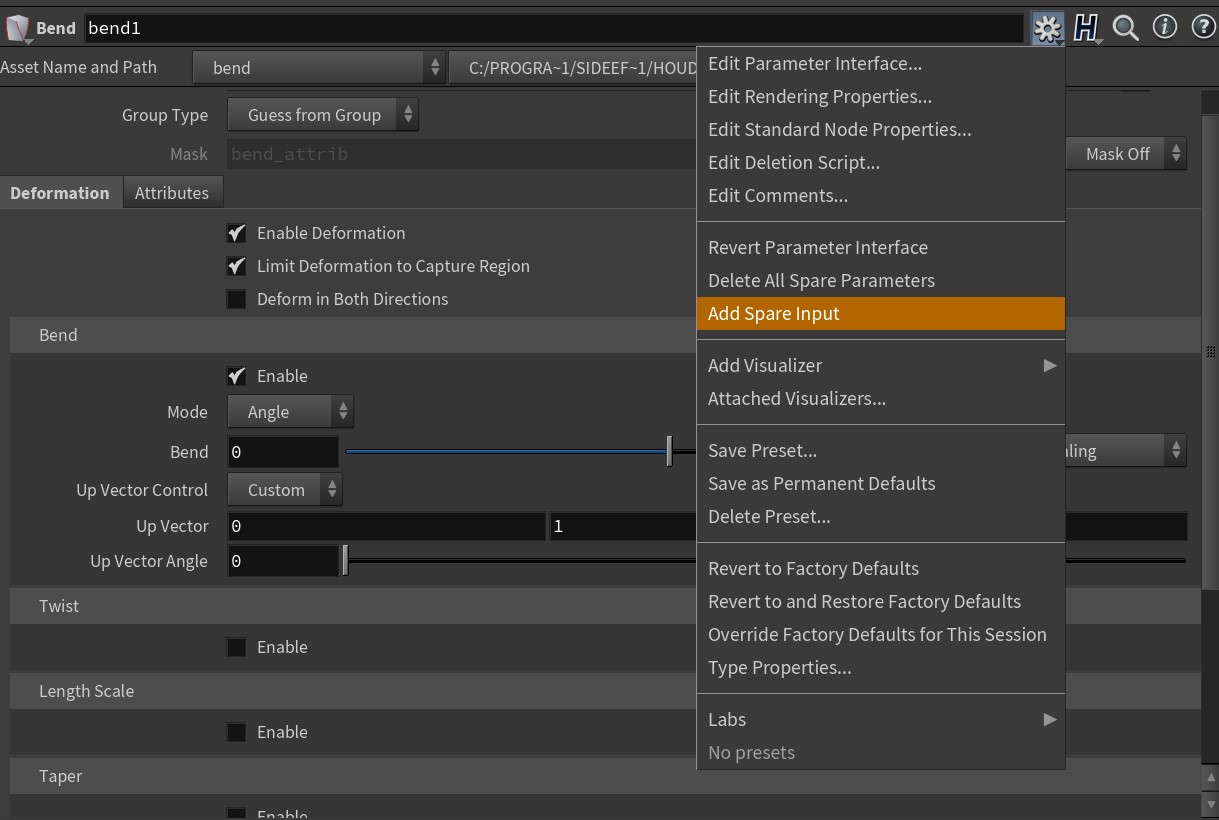
The next step, and possibly the weirdest, is to set up the Bend SOP to be able to read the bend attribute value on the current point in the loop. You’d think this would be a simple point expression, and it is, but it also isn’t. For reasons I’ll explain in a moment, what you want to do is select the Bend SOP, go to the “gear” menu in the Parameters window, and select “Add Spare Input”:

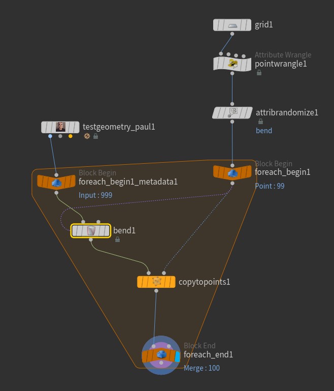
Now that the spare input is created, we need to give it the node in the loop that has the point attribute information we need. This is the foreach_begin1 node, the original Block Begin we created. Once you wire up the spare input, you’ll see a strange little purple connection flowing from the Block Begin into the Bend SOP. This lets you know that a Spare Input is connected.

Now that this connection is made, it’s time to actually vary the attribute. On the Bend SOP’s Random Seed parameter, use the following HScript expression:

point(-1, 0, "bend", 0)

This doesn’t look like much, but it’s deeply weird if you’ve been around Houdini a while and haven’t used Spare Inputs. The point HScript expression function, unlike the VEX point function, has four arguments: a SOP or input number to fetch data from, a point number, an attribute name, and an attribute index (for vector attributes, for example). For the point number, because we’re operating inside a loop where we only process one point at a time, we always want to fetch point zero, since it’s the only point that exists in each iteration of the loop. The first argument, though, is a kind of shorthand syntax that tells Houdini to use the object wired into the first spare input. If you had multiple spare inputs connected (and you can!), you could address them with -2, -3, and so on.

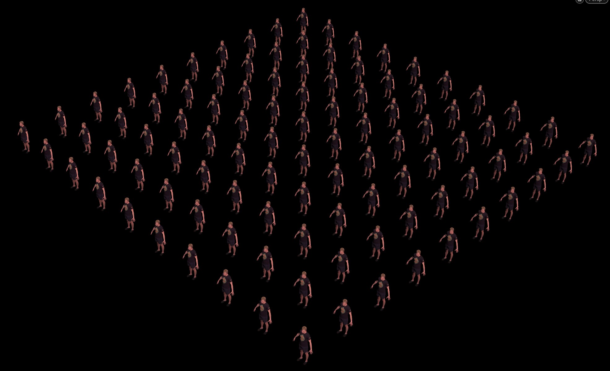
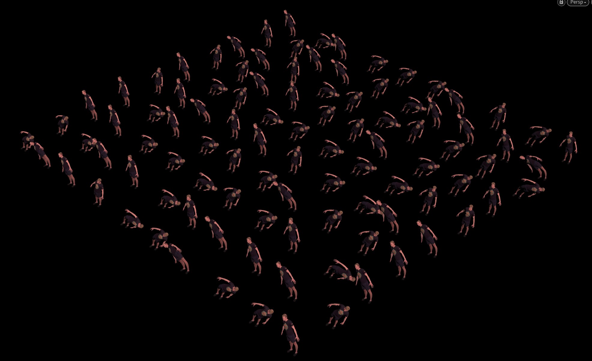
Once you’ve set this up, you’ll see that each Paul is indeed uniquely bent:

Okay, so why all the funny business with the spare inputs? It all has to do with compiled blocks. This is Houdini, so you’re not going to be satisfied with just a hundred unique bendy Pauls; no, you have to make a thousand of them in order to feel superior to all those peons using Maya or Blender or whatever. If you change that default grid to have 100×10 rows and columns, though, you’re going to see things start really crawling. This 100×10 network took a little over 15 seconds to cook and display, which really isn’t that bad considering how much work it has to do, but it really puts a damper on your interactivity (assuming you don’t run out of RAM and crash Houdini).

Set your viewport to Manual refresh to avoid re-cooking, and then drop down a Compile Block from the Tab menu. Connect the Compile Begin between the Attribute Randomize and the Block Begin, and the Compile End right after the Block End. The goal is for the little yellow container to completely surround the little orange container created by the For Each block. Next, similar to what we had to do for the For Each block, select the Compile Begin node and click the little button to create a second Block Begin node, and wire it in between the Paul SOP and the Block Begin that the Bend SOP is connected to:

The last step is to select the For Each Block End, and enabled “Multithread when Compiled”. Turn off manual mode, and you should get the same wiggly mess of Pauls in significantly less cook time!

The Spare Input method is a kind of esoteric Houdini method of keeping these nodes fully “enclosed” in a single operation that can be safely multithreaded. Regular point expressions without spare inputs will confuse the Compile Block and prevent it from actually multithreading, as will nodes that are labeled non-compilable. You can enable a little badge that tells you if a given SOP is non-compilable in the Network View Display Options, under Context Specific Badges. If your network needs to contain one of these nodes, you’re out of luck, but otherwise you can potentially speed up complex loops by orders of magnitude, especially if you’re iterating over a ton of points.

Varying Materials

Something that’s often overlooked in tutorials about copying and instancing things is how to assign different materials, or how to override material properties, on copied geometry. As with most things in Houdini, there’s a few different ways you can approach this problem, all with varying degrees of complexity and irritation. There are three basic approaches I can think of for this problem, depending on your scene requirements and your ability to withstand truly hideous sprintf commands: just make more materials, use the s@material_override string attribute, or use material stylesheets.

Just Make More Materials

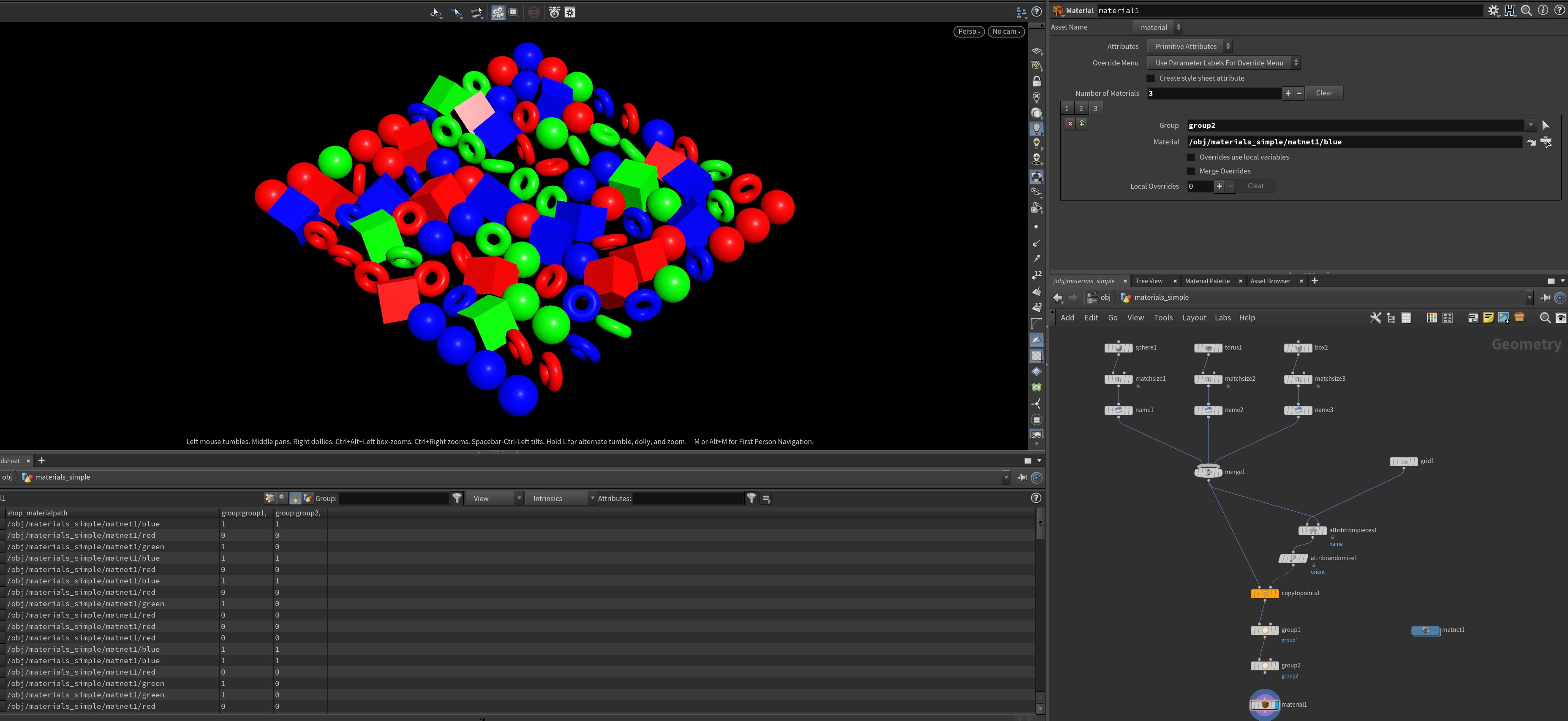
This is the simplest and most brute force approach. If you only have a few different material variants you need to work with, all you have to do is use the Material SOP to assign your materials to your various packed primitives using groups. If you check out your Geometry Spreadsheet, you’ll notice a primitive attribute that’s created by the Material SOP called s@shop_materialpath. This is the primitive attribute supported by most (if not all) Houdini render engines that determines the material assignment for a given primitive. If you don’t want to use the Material SOP, no problem! You can create values for s@shop_materialpath using VEX just like we’ve done before, using sprintf or whatever your favorite function is.

The s@material_override attribute

If you have a lot of possible variations on one or more materials, such as overriding the base color based on a point attribute, making tons of individual materials can start to be a real drag. Houdini gives you a built-in way to allow you to override any property of a material via a primitive attribute, but in true Houdini fashion, it only kind of works halfway and will generally require manual intervention.

Let’s say you have a boring old material called whatever, and its default color is red. You’ve already assigned this material to all of your packed primitives via the Material SOP or the s@shop_materialpath attribute. Your scene looks like this:

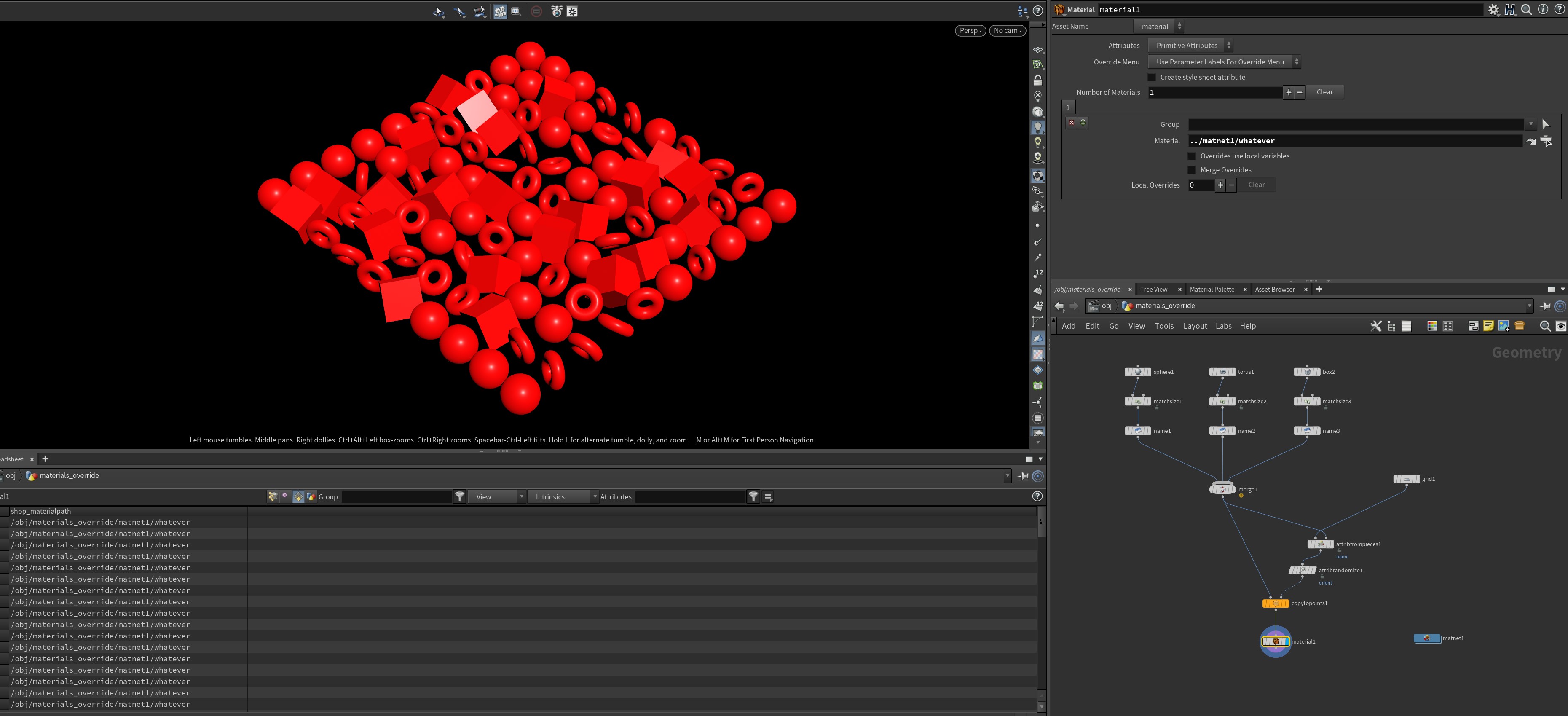
You might notice in the Material SOP’s parameter interface that there’s a multiparm called “Local Overrides.” If you hit the + button to create an override, you’ll see some extra parameters pop up, and a new primitive attribute: s@material_override, with a value of {}. There’s also a dropdown labeled “Choose Parameter”. If you click on the list, and your material has promoted parameters, you will see any available parameters to override on the list. For a Principled Shader, you can override the basecolor attribute. Changing the color value from the default to {0,1,0} turns everything green:

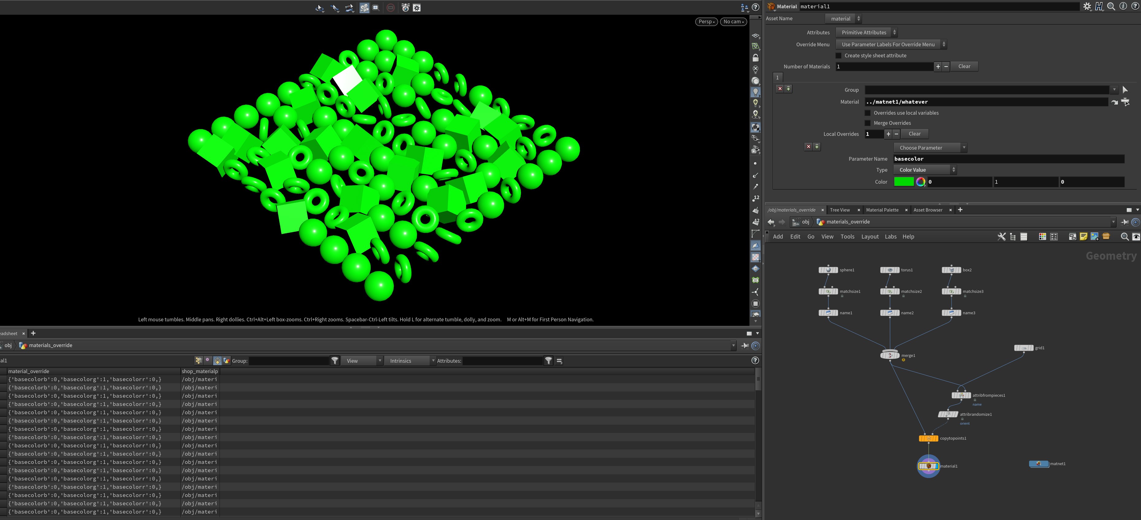
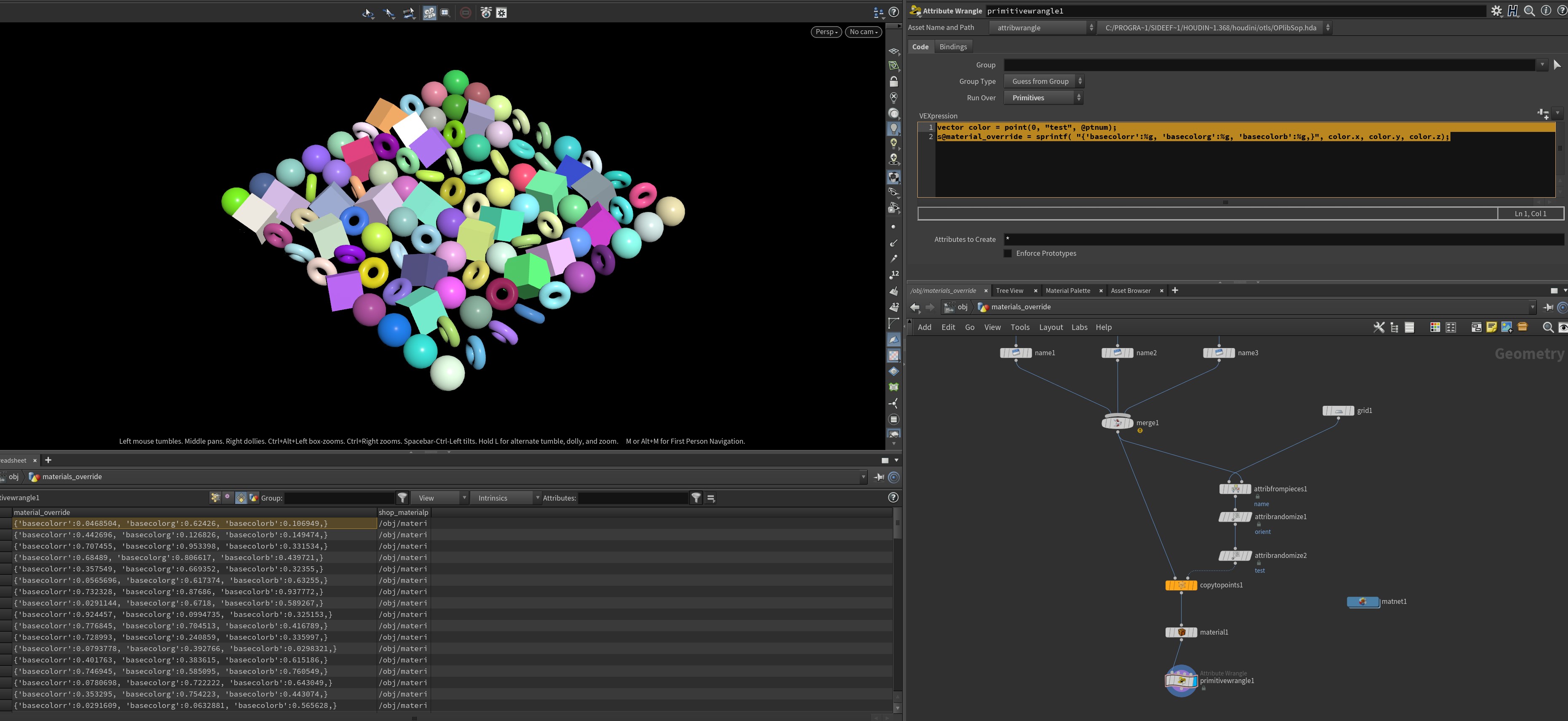
Okay, great, everything is green now. But what if we wanted different values for everything, based on an attribute? Drop an Attribute Randomize SOP on the template points right before the Copy to Points SOP, and name the attribute test. (We don’t want to use the default `Cd because it’ll confuse the viewport for our testing). You might try using point or prim HScript expressions on the color value for the override to read your attribute, but in practice, this doesn’t work, and VEX-like expressions don’t work either. So what to do about it?

Take a look again at the spreadsheet with this override enabled. The s@material_override attribute is going to have a value looking something like this:

{'basecolorb':0,'basecolorg':1,'basecolorr':0,}

This is basically a Python-like dictionary, where you have a list of key-value pairs separated by commas. A given shader property like basecolorb (the blue channel of the basecolor parameter) is defined in single quotes, and the value for that channel follows with a colon acting as a separator. The whole thing is wrapped in curly braces. If we can’t use the Material SOP to define this string exactly the way we want, it’s time again for my favorite VEX function (aside from pluralize): sprintf.

Take a look at this monstrosity:

vector color = point(0, "test", @ptnum);
 s@material_override = sprintf( "{'basecolorr':%g, 'basecolorg':%g, 'basecolorb':%g,}", color.x, color.y, color.z);

If you can stomach that syntax, you can define these overrides using VEX however you see fit, using attributes defined upstream. If you got the expression right, your viewport will suddenly look something like this:

Update: user WaffleboyTom pointed out that VEX dictionaries have a `json_dumps function that’s perfect for solving this same problem if you want something a little cleaner to read than sprintf. You just need to create a VEX dictionary and populate the keys, just like in Python, and then use json_dumps to convert it to a string, like so:

dict override;
vector color = point(0, "test", @ptnum);
override["basecolorr"] = color.x;
override["basecolorg"] = color.y;
override["basecolorb"] = color.z;
s@material_override = json_dumps(override, 2); 
// the 2 here tells vex to output this as a single-line string without defined types

It’s also very possible to accomplish generating this attribute value using Python, since it’s a Python dictionary, after all! The json module’s dumps function can convert a Python dictionary into a formatted string, so if you’d rather construct your overrides using Python, it’s sometimes a little more straightforward than doing it in VEX. Here’s what the code would look like to apply the same override:

node = hou.pwd()
geo = node.geometry()
import json
# create and initialize the material_override attribute
geo.addAttrib(hou.attribType.Prim, "material_override", "{}")
for prim in geo.iterPrims():
    # initialize overrides dictionary
    override = dict()
    # fetch "test" attribute value
    value = prim.attribValue("test")
    # set overrides
    override["basecolorr"] = value[0]
    override["basecolorg"] = value[1]
    override["basecolorb"] = value[2]
    # encode dictionary as string
    override_string = json.dumps(override)
    # set override string for this prim
    prim.setAttribValue("material_override", override_string)

Note that for this to work in a Python SOP, you’ll want to first promote the test attribute to a prim attribute. It’s a lot more code than the prior VEX example, but this is a pretty simple variable substitution… if your logic is a lot more complex than this, or if you’re trying to parse data from some external dataset, Python can often make this much easier (if a little slower to cook).

An important thing to note here is that you can only override material properties that are promoted. This means that if you just create any old material builder, throw a few material VOPs in there like a Principled Shader Core or a Redshift Material, the override won’t work. In computer science terms, a shader is a lot like a function, and a function usually has arguments such as “color” or “reflectivity” or whatever. The promoted parameters of a shader are effectively those arguments. When the shader is compiled, those arguments are left exposed so that the shader can accept values for those arguments and use them to vary the returned results. If you don’t promote your parameters, the shader won’t accept any arguments and will just run its self-contained code the same way for every object.

Another important thing to note here is that some third-party render engines (looking at you, Redshift) have certain parameters that can’t be promoted for whatever reason. For example, if you wanted to override the Filename parameter of a Redshift Texture VOP, you’ll notice there’s no inputs to the Texture Sampler that you can connect anything to, and there’s no knob icon to use for promoting. Instead, you need to create a sneaky workaround: create a Parameter VOP in the material builder and set it to be a string type, give it a name (mine’s named colortex), and then use an expression on the RS Texture VOP to channel reference that parameter:

`chs("../colortex")`

The network would look something like this:

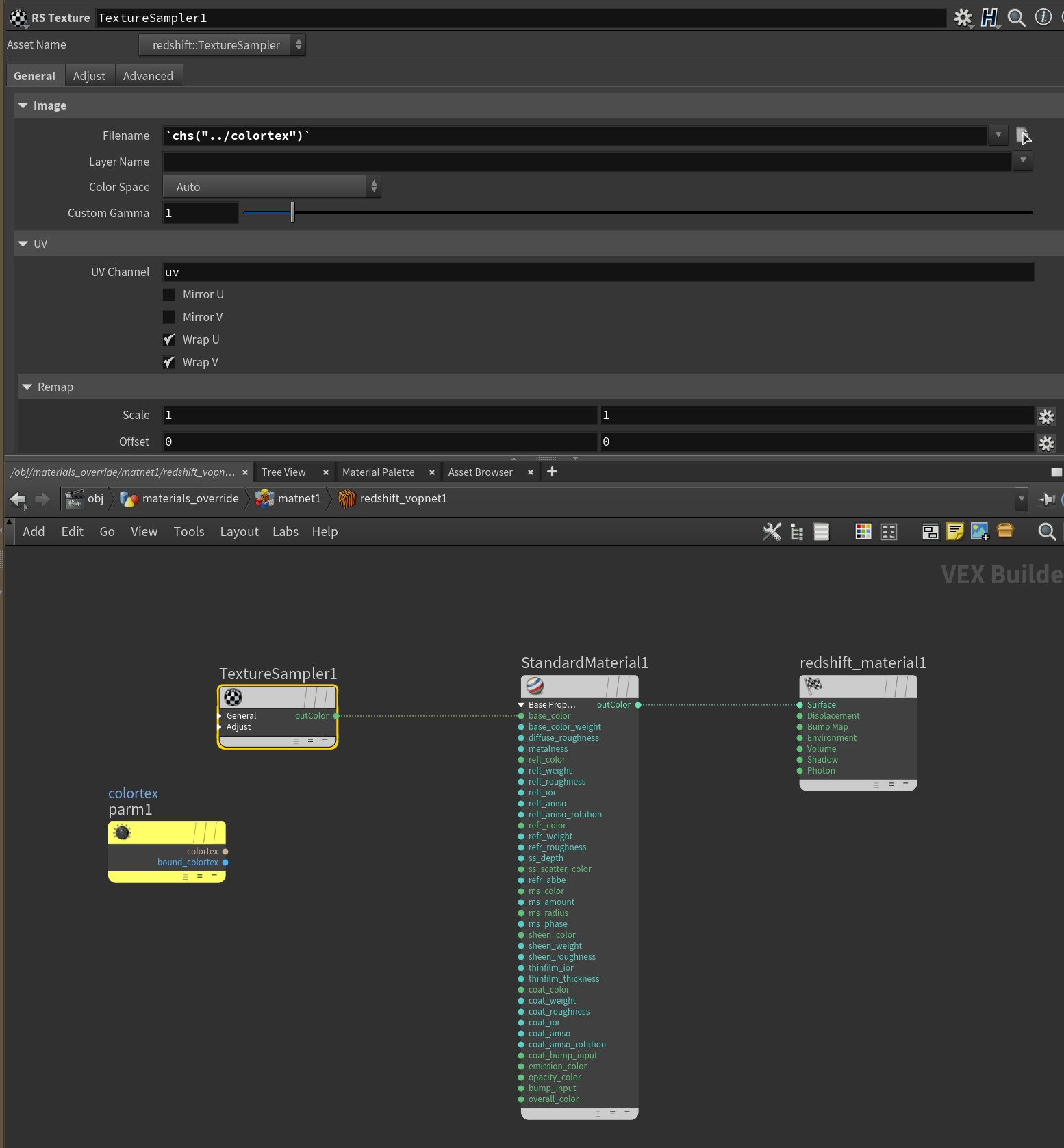
Now you can set up s@material_override to override the colortex property with a path to a texture file on disk, just like any other override.

Material Stylesheets

There’s one other way to vary material properties on instances, and that’s with material stylesheets. These were introduced several years ago as a way of being able to dynamically override material properties and assignments for objects, in addition to being able to target groups in packed and other runtime geometry. Normally you can’t do this, and it’s a very cool feature for being able to tweak materials in large crowd simulations or other highly technical scenes.

However, you should consider stylesheets to be obsolete. They are only fully supported by Mantra, and Karma has no support for them at all, because USD has no ability to evaluate them at render time. SideFX officially considers them deprecated. They can still work for doing simple material overrides for third-party engines like Redshift, but some of the fancier features involving targeting runtime geometry likely won’t work at all. If you want to learn more about how to do simple overrides using stylesheets, this article about stylesheets and Redshift gives a pretty detailed rundown. In general I don’t find that interface worth dealing with, even though it might look like less work than typing out the VEX string for overrides.

MOPs+ Attribute Mapper

If typing out all these override strings and trying to figure out the logic for what override goes where seems annoying to you, that’s because it is annoying. If you just can’t be bothered, there is a tool inside MOPs+ (the paid add-on to MOPs) that generates these overrides for you, using a custom spreadsheet-like interface. It makes it much more straightforward to lay out simple key/value pairs to associate float or integer attributes with texture paths or color values, so it works very smoothly with MOPs Falloff nodes.

If you’re curious about exactly what this tool is capable of, check out the tutorial video here to see it explained:

Solaris

brb learning solaris

Wrap-up

This ended up being way longer than I’d anticipated, but Houdini is a pretty complex beast and in my opinion it’s better to understand how Houdini is thinking under the hood than to just memorize a few patterns and then get stuck staying up all night under a deadline when things go wrong. I hope it’s helpful for you, and a welcome update to the old post that now feels a bit outdated.

Here is a HIP file showing examples of all the various copying/instancing/rotating/overriding things demonstrated in this article: https://www.toadstorm.com/freebies/toadstorm_copy_masterclass.hip

I also forgot to include a cat picture. I feel like this is one important part of the old post that I can’t leave behind, so here’s some cats:

Please feel free to berate and/or belittle me in the comments if I’ve made any mistakes. Good luck out there!