DOPs are not SOPs

I wanted to make a post about a really common misconception regarding Houdini’s geometry context (SOPs) versus its dynamics context (DOPs). Houdini’s documentation does explain a bit of basic information about DOPs, but not necessarily in the most readable way for Houdini newcomers who are first introduced to the software via the SOPs context.

Anyways, here’s the core question that’s always asked: “why isn’t [some animated property of my object] updating during this simulation?”

To understand why, we need to step back a bit to talk about the core difference between SOPs and DOPs. There are a lot of differences that are mostly too complex to talk about here in terms of data and objects and subdata and relationships and the other things that will make your head explode, but the most fundamental thing to understand is that SOPs are solved in a time-independent manner, while DOPs are time-dependent. What happens in a SOP network on frame 1 absolutely not does matter as far as frame 2 is concerned; you could cook every single frame on different machines in any order and you will always get the same result. With simulations, though, the result of frame 2 depends very much on what happened in frame 1: sourcing new objects, integrating forces, reaping particles, etc.

This means that in DOPs, by default, all you’re doing is setting the initial conditions of the simulation from SOPs. Once you make the handoff from SOPs to DOPs, the solver takes over and runs independently of anything that might be happening in the SOPs timeline.

A simple visual example

Here’s a really simple example: a POP simulation. I’m not emitting anything; just starting from a grid of points and using them as the initial geometry of the simulation. The grid of points has an animated color (Cd) attribute, driven by a noise function. I’ve copied spheres to the points for better visibility. Here’s what the animation looks like in SOPs:

Now let’s use this SOP as the Initial Geometry (think about that parameter name for a second!) for a POP Object. The DOP network in this case is minimal: a POP Object wired to a POP Solver, ending in an Output. The SOP with the color animation is assigned as the Initial Geometry.

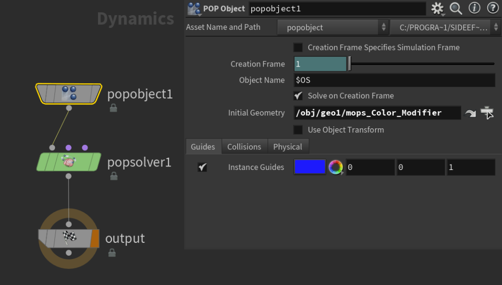
Now here’s what the resulting simulation looks like:

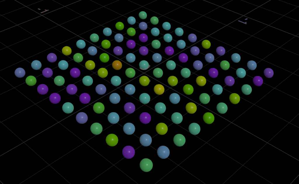
It’s very important to understand why this is happening! Or not happening in this case. The POP Object is created on the DOP network’s starting frame, which is frame 1. The Initial Geometry is sourced from the given SOP geometry at that creation frame. And then, barring any forces to integrate or other work to be done by a solver, absolutely nothing happens. You’re not giving the solver anything to do! It doesn’t care that your color attribute is animating in SOPs, because it’s not being told to fetch any data from SOPs beyond the initial state.

An even simpler (sort of) example

To give you a little more insight into DOPs, let’s strip this down even further. The SOPs animation here remains the same, but we’re going to change the DOP network to be as low-level as we can get. In an empty DOP network, create an Empty Object DOP and a SOP Geometry DOP. Set the SOP Path to the animated geometry from SOPs. Then create an Apply Data DOP and wire the Empty Object into the left input, and the SOP Geometry to the right input. This effectively applies the Geometry data from the SOP Geometry DOP to the empty DOP object we created. Wire that to an Output DOP and you should see your geometry in the viewport. Notice that it’s still not moving, for the same reason as the previous example.

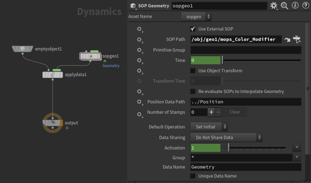
What we’re doing here is creating a generic container (the Empty Object) that has some kind of simulation data on it (the Geometry data). If you crack open the POP Object DOP, you’ll see a similar but slightly more complex network. There are all kinds of data that you can attach to an object, but by far the most common data names you’ll encounter are Geometry, which implies typical SOP geometry used in simulation such as particles or RBDs or Vellum cloth, and ConstraintGeometry, which implies constraint primitives used by RBDs and Vellum. The various solvers in Houdini know to look for data of these specific names, look for attributes on that data (like v, w, restlength, and so on), and then use those attributes to integrate physical forces or other effects.

Updating data from SOPs

Now we want to get that animated color attribute in here. To do this, we need to instruct the DOP network to fetch the data from SOPs that we want, and apply it to the Geometry data of our simulation. The most straightforward way to do this is via the SOP Solver DOP. Create a SOP Solver DOP and a Multiple Solver DOP. The Multiple Solver is a convenient little node that you can wire an object into on the left (in this case, the output of the Apply Data DOP), and any number of solvers on the right (in this case, the SOP Solver DOP). The network now looks like this:

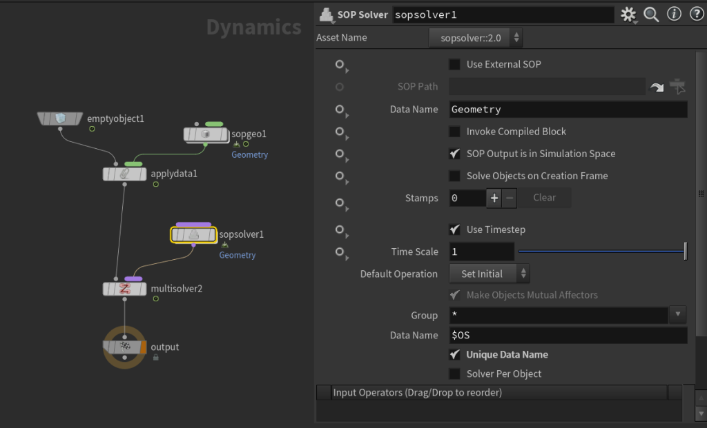
If you take a closer look at the SOP Solver parameters, you can see that the default Data Name is Geometry. That means that anything that happens inside the SOP Solver will impact the Geometry data of the object, which is perfect because that’s what we’re seeing on the screen. Dive inside the SOP Solver and you’ll see something a little different:

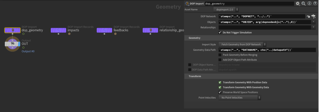
The default stamps expressions here are a bit spooky, but they’re basically just telling this dop_geometry node to fetch whatever we told it to fetch from the object we’re connected to. If you middle-mouse click on the Geometry Data Path parameter, you’ll see the expression evaluates to Geometry. Also take a closer look at the node type of this node… it’s a DOP Import SOP. We’re back in SOPs! That’s the magic of this solver… we can take geometry-like data from a DOP object and manipulate it using SOP tools, in the middle of a simulation.

In this example, what we want to do is get the animated Cd attribute from our original SOP timeline and apply it to our simulated geometry. Now that we’re back in SOPs, we can start to think in SOP terms again! How would you copy an attribute from one SOP to another…? You’d just merge that source geometry in from another network and use the Attribute Copy SOP!

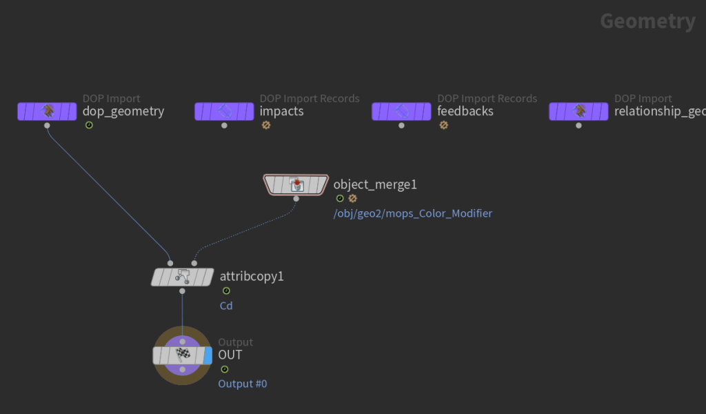
If you play this back, you’ll see that now the colors are again animated as before.

Getting a little more complex

The SOP Solver DOP is incredibly powerful and intuitive once you understand what it’s doing; you can manipulate pretty much any aspect of the simulation during runtime using all the SOP tools you’re likely already familiar with. The only big downside is that it tends to have a bit of overhead. In this example you won’t really notice much, but if you start updating attributes on a much heavier simulation, you’ll notice a significant slowdown.

If all you need to do is update attributes and not actually use SOP tools, there’s a much faster way to do it: the Geometry Wrangle. Unfortunately for those of you who are scared of code, this requires that you use a bit of VEX, but it’s really nothing too crazy for most cases. Disconnect the SOP Solver and wire up a Geometry Wrangle DOP in its place. What we want to do with the VEX is grab the Cd attribute from the SOP geometry using a point() expression, and then bind it to Cd. This is pretty straightforward:

vector Cd = point(1, "Cd", @ptnum);
v@Cd = Cd;

If you’re used to Point Wrangles in SOPs, this syntax will look familiar. But what is input 1 in this case? We don’t have the usual four inputs on the node itself to use in DOPs, so instead you have to go to the Inputs tab and configure it there:

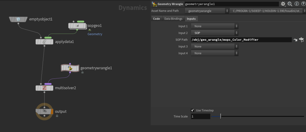
Remember that the input numbered 1 in a Wrangle is referring to the second input, or Input 2 here. This is because in VEX terms, the inputs are an array starting at index 0, even though the UI labels them as inputs 1 through 4. This has always been confusing. The configured Input 2 shown above is what we’re referencing when we run that point(1, "Cd", @ptnum); line.

Finally, take a look at the Data Bindings tab. You don’t need to change anything here just yet, but this is where you’d set the name of the DOP data you intend to modify. By default this is Geometry which is exactly what we want. We’ll come back to this later. With that code in place, run the timeline and you will again get the glorious animated color attribute you’d always dreamed of:

Getting weirder

Most people encounter the problem at the root of this blog post because they want to make silly wiggly Vellum things like they saw on Instagram or whatever. The way these are done is typically by manipulating the restlength or stiffness of various Vellum constraints to cause them to inflate or droop or anything you like. Where people get stuck is that they try to use some attribute they’ve carefully animated in SOPs to drive the constraint animation, not realizing that DOPs absolutely does not care about all the work you’ve done. Let’s do an example of this now where we take the techniques we’ve already learned and apply them to a slightly different bit of simulation data, ConstraintGeometry.

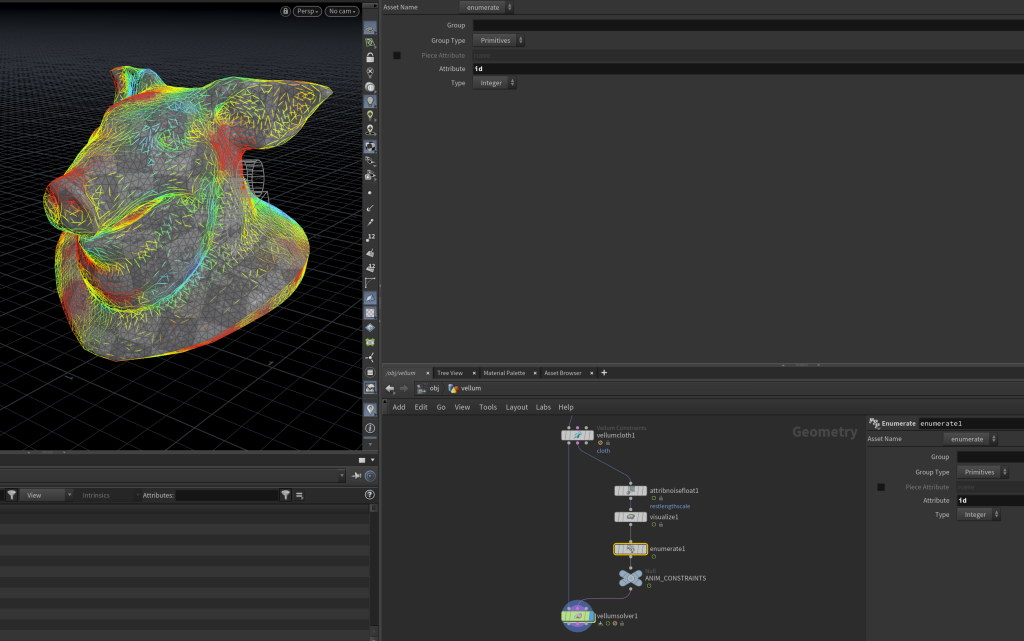
Here’s a really simple Vellum setup. A remeshed pig head gets fed into a Vellum Configure Cloth SOP, with the stretch stiffness set pretty high: 1e+10. Following that, some animated Attribute Noise is used to create a float attribute on the constraint primitives called restlengthscale. The value is set to a minimum of 0.0 and a maximum of 2.0. This attribute is not actually one recognized by the Vellum solver… we could name it catvomit and it would have the same effect here. There’s also a Visualizer here to be able to better see the generated noise pattern. Finally, an Enumerate SOP is added here to create an id attribute on the constraint primitives. If you’re going to be manipulating constraints inside a Vellum Solver SOP, it’s very important that you have a primitive id attribute on the constraints because the constraint primitive order will be scrambled in the simulation due to all of the behind-the-scenes prep work that the Vellum Solver SOP handles for you. This isn’t necessary if you’re using an old-fashioned DOP network, but having an id on your primitives is still good practice! The network looks like this:

What we need to do now is bring this restlengthscale (or catvomit) attribute into DOPs. It’s very possible to do this with a Geometry Wrangle just like before, but Houdini has a convenience node for you called Vellum Constraint Properties that makes setting certain properties like restlength much simpler. Unlike restlengthscale, restlength is actually recognized by the Vellum solver and will affect the constraint primitives.

If you dive inside the Vellum Solver SOP and place a Vellum Constraint Properties node, you’ll see the familiar Bindings and Inputs tabs at the top. This is because internally this HDA is a Geometry Wrangle (it’s actually a Geometry VOP but close enough) with some shortcuts set up for you! Under the Bindings tab you can see that the Geometry parameter is set to ConstraintGeometry, so this operation will affect the constraint primitives and not the actual cloth primitives.

Now under the Inputs tab, we want to again point to a particular SOP to fetch data from, just like before. Inputs 1 and 2 come pre-configured and we have two extra inputs anyways, so just set Input 3 to be a SOP and point it to the animated constraints in your SOP network. It’s important when using these nodes inside a SOP wrapper like the Vellum Solver SOP (as opposed to a DOP Network) to always use SOP paths rather than context geometry. The context geometry is meant to point to the inputs of the DOP network, but because the DOP network in this case is wrapped up in a SOP, it’s not going to point you to the input you’re expecting. Just use SOP paths.

Finally, we need to go to the Properties tab and modify the Rest Length Scale. We want to only affect the stretch constraint group, so enable the Group parameter and give it the stretch group so we don’t change the bend constraints. Since we’re changing the rest length per-primitive we’ll leave the constant value at 1 and enable Use VEXpression. The VEXpression needs to do essentially exactly what we did before with fetching a point attribute, but instead we’re fetching a primitive attribute and we need to use the primitive id attribute rather than just the primitive number. The code looks like this:

// get the matching primitive from SOPs based on id
int primnum = idtoprim(2, i@id);
// get the attribute we made in SOPs from this prim
float scale = prim(2, "restlengthscale", primnum);
// override the Rest Length Scale parameter with this value
restscale = scale;

If you’re not used to VEXpressions, the property we’re overriding, restscale, is the name of the parameter we’re setting values for on the Vellum Constraint Properties DOP. Under the hood, this node is reading that value and using it to set the restlength primitive attribute, based on the restlengthorig primitive attribute that’s automatically created. We could do this ourselves with a little arithmetic but this node just simplifies it for you.

Here’s the result from animating those constraint lengths:

Incidentally, this whole process of importing an attribute from SOPs based on an id or name and binding it to some DOP geometry property is something I’ve simplified somewhat with MOPs+ Fetch Attribute. If you don’t feel like going through that whole process every time, or if you need to sneak a quick remap in there, it handles much of this for you.

Houdini (sometimes) will help you!

There are a few exceptions to this rule, mostly related to RBDs. If you look at the RBD Packed Object DOP, there’s an optional “Overwrite Attributes” parameter and a list of attributes you can overwrite. This is a shortcut to fetch attributes from your chosen Geometry Source (usually a SOP) and update them during the simulation. Similarly, RBD-specific attributes like i@deforming can force affected geometry to update its collision mesh based on any deformations happening in SOPs, and i@animated has a similar effect for animating the transform of each object. Shortcuts like this are the exception rather than the rule in Houdini, though, and it’s important to know that most of the time you’re responsible for updating the DOP geometry from SOPs.

Remember: DOPs are not SOPs

If there’s anything to take away from this article, it’s that SOPs and DOPs have their own timelines. If you want your simulation to have animated attributes from SOPs, you just have to fetch them yourself. Take the opportunity to play around a bit more with SOP Solver DOPs and Geometry Wrangles, though, because you really can mess around with just about any aspect of your simulation and create some really unexpected effects.

Here’s the .hip file, and hope this was helpful!